
The 3D Editor
Drawing a cell in three dimensions — boxes, cylinders, faces, booleans, fillets, STEP parts, placed cells, bond wires and ports — in circuitRF's own 3D editor, which needs no solver to draw anything. Taught through two examples, an MMIC in a lidded package and a coaxial connector launching onto a board.
The 3D editor is where a cell's 3D view is drawn: solids, sheets, bond wires and ports in three
dimensions, with the cells they are built from placed inside them. It is part of circuitRF. It is not
a front end to Palace or openEMS, and it needs no solver installed. Everything on this page up to
Simulating — drawing, editing, placing cells, wires, ports, setups, check, explain and
section pictures — works on a machine with no 3D solver at all. A solver is needed for one thing: pressing
Run. When you do, circuitRF offers to install the one the setup names (see
3D EM ▸ Getting the solvers), and EM Solvers says which one suits
which problem.
This page teaches the editor through the 3D Package example — an MMIC die in a ceramic package with a lid — which was drawn with exactly the gestures below. Open it with File ▸ New ▸ Examples ▸ 3D Package. The 3D Connector example teaches the operations the geometry kernel adds — booleans, fillets and STEP parts — through a coaxial connector launching onto a board (below).
The 3D view of a cell
A cell can have up to four views: a schematic (what it does), a symbol (how it is placed in a
schematic), a layout (its artwork, layer by layer) and a 3D view (its solid model). The 3D view is
a file of its own, <cell>/3d/<name>.c3d, a small JSON document you can read and diff, and the Project
panel lists it under the cell like the others. File ▸ New 3D Design… makes a cell with an empty one,
New 3D View on a cell's menu in the Project panel adds one to an existing cell, and New 3D View from Layout makes one
holding the cell's own layout, ready to extend — the quickest way to take a layout you have already set up
for EM into 3D. It brings in the layout's port labels as the 3D view's own ports, each the sheet a 3D run of the
layout would build: with the layout's 3D setup when it has one, else with a default driven setup, which a message
says. A port you do not want is deleted like any other.
When the layout was made from the cell's schematic (Update Layout from Schematic), the new 3D view also gets one VAR
per name that drives it — each cell parameter, and each VAR of the schematic at its current value — linked by name,
so a dimension written with w50 follows the schematic's w50 when the cell is simulated by EM in 3D. See
EM cells.
The 3D view's ports are its own from then on, each remembering which placed layout and which of its port labels it came from. When a placed layout's port changes afterwards (its Width or Use edge width, or where its label is), opening the 3D view, or saving the layout while it is open, posts one message per port that no longer matches; nothing is rewritten. A port whose label has moved is usually refused, drawn only as a red outline that cannot be clicked. Update Ports from Layout — on the port's row in the object tree, on the placed layout's row, and on the view's own right-click menu while any port is out of step — replaces those ports with what the layouts build now and brings in any label no port stands for yet, as one step you can undo. Two placed layouts often both number a port 1: the later one's comes in at the next free number, and the Messages panel says which became which. Ports the layouts do not state are left alone.
A port's Number… and Name… are on its right-click menu, in the canvas and in the Object Tree. A number another port already uses is refused; a default name such as P3 follows the new number, and a name you gave is kept. A renumbered port still knows its layout label.
- What it holds. Boxes, prisms, cylinders, spheres, sheets, polyhedra and bond wires, each made of a named material; instances of other cells' layouts or 3D views; ports; boundaries on faces; VARs; and any number of EM setups. Everything a 3D solve needs is in the one file.
- Units. Every coordinate is stored as a whole number of database units (DBU; 1,000 per µm by default), exactly as a layout's are, so nothing drifts when you save and reopen. The display unit — the unit you read and type in — is chosen with the Unit box on the toolbar. It starts as the cell layout's unit, or the technology's. Changing it moves nothing. The example is drawn in mil; its die's layout is in µm. Both are exact.
- Materials come from the cell's technology. Assign Material…, New Material… and the Edit… button
beside the Inspector's Material box open the Materials dialog: every material the technology has — its own and
its libraries' (
.cmatfiles, see File formats) — with every property of the selected one on one form: dielectric, conductor, thermal, the σ(T) and k(T) tables, colour, appearance and notes. See, edit, Duplicate or make one there, then assign it. Edits go to the file each material belongs to when you press OK, as an unsaved change there — save that file to keep them; Cancel discards them. Delete (or right-click a material) removes one; a material already in use is listed with its uses first. A material that already exists is renamed in its own file's editor, which renames it everywhere it is used (Materials walks through the editor and how a.cmatrelates to a.ctech). A placed cell brings its own technology's materials with it — see Hierarchy. - Built-in materials. The package button beside Duplicate lists the materials circuitRF ships with (metals,
substrates, glass, die-attach and thermal materials) below the technology's own; each carries the package mark at
the right of its row, and a material the technology already names is not listed twice. Assigning a built-in
material, or editing any of its properties, copies it into the list shown under New, duplicated and built-in
materials go to — usually the technology's own
.ctech— where it is yours to change from then on, and the mark goes. A built-in material keeps its name; Duplicate it to make a copy under another. The technology editor's Materials tab has the same button. - Edit Material… opens the file a material is defined in, on its row. Right-click a material's heading in the
Objects tree (by material; No material has none), or an object's row, which says which material:
Edit Material 'FR4'…. A material in the technology's own list opens the technology on its Materials tab; one
from a
.cmatlibrary opens that library. A library shipped inside circuitRF is not a file you can edit, so its material opens on the technology's Materials tab, where it can be read. A placed cell's part edits its own technology's material, and the item names that file: Edit Material 'Au' (in pa.ctech)…. An editor that is already open — in another tab, floated, or in another workspace window — is brought forward rather than opened again, and the list scrolls to the row. With no technology, the item is greyed; give the design one with 3D ▸ Materials…. - Hovering an object names it and shows the material properties that apply to what it is to the solver: a conductor, a wire, a via or a sheet shows σ at the operating temperature (and μr when it is not 1), never εr or tanδ; a dielectric shows εr (or its three tensor values) and tanδ, and σ only when it is above 0 — a doped substrate's loss; air says Air. What the object is follows its Role when you gave it one, as the solve does. An object with no material says so, and a material that states nothing says that. With a thermal setup active, every solid also shows k, and ρ and c when the setup computes a Z_th or a pulse.
- The editor and the viewer are one pane. The 3D view a solver result opens in, Show 3D on a setup, and this editor share the camera, the clip plane, the mesh and field displays, and every key described in 3D EM ▸ The 3D view. The editor adds the drawing.
The camera is the viewer's: middle- or Alt-drag to orbit; Shift-drag to pan; right-drag or scroll to zoom (with Use Hertzon interactivity off: drag to orbit; right-, middle-, Alt- or Shift-drag to pan), or Ctrl/Cmd+= and Ctrl/Cmd+−; the arrow keys pan and Shift+arrow orbits; Home or Ctrl/Cmd+0 fits, Ctrl/Cmd+E fits the selection; 1 is isometric, 2–7 the six orthographic views, P toggles perspective, L the realistic view; C turns on the clip plane. A new 3D view opens orthographic. The line along the bottom of the view is the status line: what the armed tool wants next, or what the last edit did, or why it was refused.
The example: an MMIC in a package
File ▸ New ▸ Examples ▸ 3D Package copies a workspace with two cells to a folder you choose, and opens its
README.md, which carries the numbers quoted here.
- Thru die — an MMIC's layout, drawn in µm on a GaAs technology (
tech/mmic-gaas.ctech: 100 µm of GaAs, two gold metals, a gold back side). A 1000 × 600 µm die with a 75 µm line between two 100 µm pads. - Package — a 3D view, drawn in mil on a ceramic-package technology
(
tech/ceramic-package.ctech: alumina, gold and a lid alloy). A gold floor; 5 mil of alumina on it; a gold die-attach pad on four gold vias; two 5 mil gold leads; the Thru die layout placed on the attach pad as instance U1; a ball–wedge gold wire from each die pad to its lead; a port at each lead's outer end; four gold walls; and a lid.
The cavity is 400 × 320 mil and 40 mil high — three cell parameters, cav_w, cav_l and cav_h,
that the floor, the base, the walls and the lid are all written in terms of, so changing one redraws the
package (see Dimensions as expressions). The die, its pad, the leads, the wires and the
ports do not depend on them: a bigger cavity leaves the die where it is and moves the walls out.
The second example: a connector launch
File ▸ New ▸ Examples ▸ 3D Connector is a coaxial connector launching onto a 50 Ω microstrip at a board's edge — the 3D problem an RF board meets most — and it is built from the operations the geometry kernel adds:
- Board — a layout in mil: 20 mil of PTFE-glass laminate over a ground plane, with a 62 mil line.
- Flange — a 3D view in mm: a plate with a hole, a Subtract of a cylinder from a box. It is the source of the STEP file below, standing in for the model a connector's maker would send.
- Launch — a 3D view in mm: the board placed from its layout; a housing with its bore subtracted and
kept as the PTFE fill (Keep tools); the flange imported from STEP (
flange.step, exported from Flange) and united with the housing; a centre pin whose tip is filleted — a fillet on a curved edge; and two ports and two setups, one for Palace and one for openEMS.
Its README.md lists the gestures that drew it, in order — Box, Cylinder, Boolean ▸ Subtract… with the Tool
selected first and Keep tools ticked, Export STEP… and Import STEP…, Boolean ▸ Unite…, E and
Fillet… — and what each run measured. The experiment it exists for is one click: untick Enabled on the pin's
fillet row in the object tree and Simulate again. Palace meshes the fillet as a curved surface; openEMS, whose grid
cell at the tip is wider than the fillet's radius, says before the run that it will not represent it. What each
makes of it is in EM Solvers ▸ What each solver sees of curved geometry.
Selecting
O, F, E and V choose what a click selects — a whole object, one face, one edge, or one vertex — and the toolbar has a button for each. What is under the cursor is highlighted; a click selects it, Shift-click adds or removes, Esc clears.
Edge mode (E) picks the edge nearest the cursor that you can see. An edge is a whole run between two faces — a cylinder's rim is one edge, not a ring of segments — named by those two faces:
xmax|zmax,bottom|side,bore:side|zmax. Where one pair of faces meets in more than one place the name takes a number,side|zmax|1,side|zmax|2, counted in the object's own frame, so moving or turning it renames nothing. Double-click an edge to take its tangent chain — every edge that carries on smoothly from it (within a degree), the loop round a rounded top — and Shift-double-click to add it; a chain that meets a fork stops there and says how many ways it could go. Properties shows an edge's faces, kind and length, and a circle's or an arc's radius and centre; several edges, their count and total length. Edge mode needs no geometry kernel.B selects the next thing behind the selection along the line of sight through the cursor, and Shift+B steps back toward you; the status line says where you are (
Face zmin · "base" · 2 of 5). In the example: select the lid in Object mode, press B, and the selection passes through the lid to the wire, the die and the floor in turn — the way to reach something inside a closed package without hiding anything. A face's boundary — the blue or green tint of a thermal one, the tint of an EM one — is what a click on it selects (its row, and its fields in Properties); B from it steps to the solid, or in Face mode the face, under it.Right-click opens the menu for what is selected: Hide, Isolate, Show All, Select Owning Object, and the commands this page describes. A right-click anywhere over the selection keeps it, even where something stands in front of it, since a selected face shows through what covers it; anywhere else it selects what is under the cursor first. To act on the thing in front, left-click it first. Hide the lid and the walls to work inside the package; Show All brings them back. Hiding changes only the picture — the solver still sees everything.
H hides the selection, and shows it again: press it in the view or in the object tree (where a selection of several rows is usually made), or use 3D ▸ Hide / Show Selection, the same item on either right-click menu, or the eye button on the toolbar just left of the mesh button. When all of the selection is shown, H hides it; when all of it is hidden, H shows it; when some of it is hidden, H shows all of it first, and the next H hides all of it. The selection stays selected while hidden, so a second H brings back exactly what the first took away. A group selected whole counts as its members, and records count as well as objects (a probe, a mesh region, a thermal boundary, a symmetry plane, a field plot), each hidden as its own tick hides it. An object's hide is one undo step and is saved; an instance's parts are hidden in the view only. The eye button's background shows the state: the accent colour when all of the selection is shown, the same colour dimmed when some of it is hidden, and none when all of it is hidden; with nothing selected the button is greyed. Its tooltip says what a press will do. It is in a setup's 3D view too, where hiding lasts for the session, as that view's ticks do.
The Objects tree lists everything by material or by type — and your groups first; a click there selects in the view, and the Properties panel shows the selection's name, material, dimensions and position, every one of them editable. The eye buttons in its header hide or show every row it lists, records included — heat sources, probes, mesh regions, effective blocks, symmetry planes, thermal boundaries and field plots — as one undo step. An object's tick is saved with the document; a record's tick (a place, a boundary, a plane) is this view's alone.
Snapping
The cursor snaps to a vertex (a square marker), an edge's midpoint (a triangle), the nearest point on an edge (an ×), a face's centre (a circle), and otherwise to the grid (a small +) on the drawing plane. A vertex wins over anything else within reach. Snapping reaches into placed cells: the corner of a pad on the die, inside U1, is a target in the package. Only what you can see is a target, except through a translucent object or with the clip plane on.
The magnet button turns snapping off and on, and the buttons beside it turn each kind on and off; these are your settings, not the document's. Hold Alt (Option on a Mac) to suspend geometry snapping while drawing; the grid still applies. The Snap box beside Unit sets the grid step (the example uses 0.5 mil); changing it moves nothing already drawn. A ≈ before a coordinate means the point is not exactly on the database-unit grid (a corner of something rotated by an odd angle).
Tracking from a point. While a tool is armed, rest the cursor on a snap point (a vertex, a midpoint, a centre) for half a second: a small green + marks it as a reference. Move away and the cursor locks onto the lines through it along x, y and z, drawn dashed in the axis's colour, with a diamond marker on the line. Near an edge the point stops where the line meets that edge; elsewhere it moves along the line in grid steps. Two references give the point where their lines cross, such as the x of one corner and the y of another. This lets you draw a sheet from a trace's corner straight down to a ground plane that has no vertex beneath it: rest on the corner, then move down to the ground's edge. A vertex under the cursor still wins. Resting on a reference again removes it. A reference is forgotten after ten seconds unused, and when the object is finished or the tool is put away. Alt (Option) suspends tracking along with geometry snapping.
Drawing
The drawing plane. Shapes are drawn on a plane — XY, YZ or XZ at an offset along its
normal — chosen from the toolbar's plane box and offset field (a bare number is the display unit; 25um
or 10mil says its own), from 3D ▸ Drawing Plane, or from geometry: with a tool armed, Ctrl-click
(Cmd-click on a Mac) a face to draw on it, or Ctrl/Cmd+Shift-click a snapped point to move the
offset there. A faint grid lies on the plane; moving the camera never moves it.
The tools are on the toolbar, under 3D ▸ Draw, and at the cursor: press Shift+A, then one letter.
| Letter | Tool | Clicks |
|---|---|---|
| B | Box | a corner, the opposite corner, then the height |
| S | Sheet | two corners (a conducting rectangle with a thickness) |
| G | Polygon | a click per vertex; click the first, press Enter or double-click to close |
| L | Polyline | construction lines, never solved; Enter or a double-click ends one |
| Y | Cylinder | the centre, the radius, then the height |
| E | Sphere | the centre, then the radius; it is centred on the drawing plane |
| O | Ellipsoid | the centre, then one radius; its three semi-axes start equal and are set in Properties (see Phantoms) |
| P | Port | two corners on the plane (see Simulating) |
| C | Lumped element | two corners across a gap, as a port (see Simulating) |
| W | Wire | two pads, then the loop height (see Bond wires) |
| H | Heat source | two corners on the plane, then its name and power (see Temperature) |
| T | Probe | a click on a face: the temperature there (see Temperature) |
| M | Mesh region | a box, then the element size inside it (see Temperature) |
Typing instead of clicking. While a shape is in progress, type a digit and a box opens at the cursor
showing what the next click would set — width and depth, then height (or radius, then height). Tab
moves between the fields, Enter accepts, Esc goes back to the mouse. A value can carry its own unit
(127um while drawing in mil) and can be an expression (see Dimensions as expressions).
Each new object takes the toolbar's material and a name you can change (box1, cyl1, …), and each is one
undo step. Esc cancels a shape; pressed again it puts the tool down.
How the example's package was drawn. With the material box on Gold and the XY plane at 0, Shift+A
B, one click anywhere, then typed: cav_w + 2*wall Tab cav_l + 2*wall Enter, floor_t
Enter. That is the floor's size; its corner was typed in Properties (-cav_w/2 - wall,
-cav_l/2 - wall, -floor_t), and its name (floor) there too. The alumina base, the attach pad, the
leads, the walls and the lid are drawn the same way. The four vias are one cylinder (radius 2, height
5) and Array… (right-click): 2 × 2 at 36 × 20 mil. The walls and the lid were drawn last: drawn
first, they would hide the inside while you work on it.
Extrude (a sheet's menu, 3D ▸ Modify, or a polyline selected in the tree) pulls a closed polyline, a polygon or a rectangle into a prism: move to set the distance and click, or type it. K keeps the source.
Phantoms
A phantom is a body for SAR work, made of nested layers, each its own material. 3D ▸ Draw ▸ Phantom offers six:
| Phantom | Layers, outermost first | Starts as |
|---|---|---|
| Head (3 ellipsoids) | skin, skull, brain: concentric ellipsoids, each shell taken off every semi-axis | openEMS's head phantom: semi-axes 100, 80, 100 mm, shells 9 mm |
| Body (3 cylinders) | skin, bone, tissue: coaxial cylinders of one length | openEMS's body phantom: radius 100 mm, 260 mm long, shells 8 and 10 mm |
| Flat Phantom | shell, liquid: the liquid in an open-topped box, the shell on its floor and four walls | 300 × 200 × 152 mm outside, a 2 mm shell, 150 mm of body liquid |
| Generic Head (circuitRF's own) | ear-left, ear-right, shell, liquid: an ellipsoid shell of head liquid with a flat ear spacer each side | semi-axes 100, 78, 115 mm, a 2 mm shell, spacers 4 mm thick and 25 mm in radius |
| Sphere, Box | one homogeneous body | radius 50 mm; a 100 mm cube |
A phantom is one object: it moves, turns, hides and is left out of the solve as one, and the tree shows its
layers under it. Where layers overlap the innermost wins, so the brain is brain, not skin. Properties
shows only the dimensions its shape uses — semi-axes, radius and length, or size, and the shell thicknesses —
and one material per layer under Layers, outermost first. The layers start as the tissue library's records
of those openEMS phantoms (Add Tissue Materials, in the technology editor or at the top of the Materials dialog a layer's New Material…
opens, puts the library beside the technology; see Materials); the flat phantom and the generic head start in the tissue-simulating
liquids and circuitRF's own shell material. Every
layer is solved as a lossy dielectric. Flatten Phantom (its menu) replaces it with one ordinary solid per
layer, <phantom>_<layer>, in a group named after it; the solve is the same.
What each phantom's dimensions are drawn from, and the tissues that fill them: Tissues and phantoms.
A sheet on a cylinder is a strip of zero thickness on the cylinder of one radius about x, y or z — a birdcage
coil's rung or end ring — written in the .c3d as a CylinderSheet (circuitrf reference 3d has its fields:
the axis, a point on it where the strip starts, the radius, the length along the axis, and the azimuth it starts
at and sweeps through, in degrees). There is no tool to draw one; the 3D view draws it as written. Only openEMS's
cylindrical grid about the same axis solves it (A cylindrical grid); every
other solver refuses it by name.
An ellipsoid on its own (Shift+A O) is a centre and three semi-axes along its own x, y and z, so turning it turns its axes. Its surface is curved: face edits, fillets and boundaries are refused on it, as on a sphere.
Moving and editing
Whole objects (Object mode; right-click, or 3D ▸ Modify). 3D ▸ Modify is greyed out until something is selected, and each item in it is enabled only when it can act on the selection — the same rule the right-click menu follows, where a greyed-out item's tooltip says why:
- G moves the selection: click a base point, then a target point, both snapped — two clicks put one corner exactly on another. X, Y or Z holds the move to that axis, Shift+X/Y/Z to the plane across it; type a digit for the distance.
- R rotates about the drawing plane's normal in 15° steps (Shift for free, or type the angle); Rotate 90° and Mirror act at once. A rotated box is still a box.
- Ctrl+D (Cmd+D) duplicates and moves the copies; Array… makes copies along up to three axes at a pitch, previewed as you type; Align lines objects up on an axis.
- The gizmo at the selection's centre: drag an arrow to move along it, a square to move in its plane.
- Order: where two solids overlap, the later one in the list wins the shared volume — except that metal always wins over a dielectric, whatever the order. That is why the example's vias can simply be drawn through the alumina base: they are gold, so they win.
Faces and vertices (Face mode, F; Vertex mode, V):
- N (Move Along Normal) pushes or pulls a face. Its neighbours keep their planes and stretch to meet it, so a pushed box is still a box. It stops before a neighbour would vanish, and says which.
- G moves a face freely (its neighbours tilt to follow), or a vertex in Vertex mode; Properties' Set coordinates types where a vertex goes.
- A polygon sheet, a prism or a polyline lists every point in Properties as x, y and z in the display unit, with the length of the edge to the next point; type one and press Enter. A sheet's or a prism's points stay on its plane, so the coordinate across the plane is greyed (Offset moves the whole outline), and a prism's list is its bottom, with the top following. A polyline's point may leave its plane.
- Shift+E grows a new solid out of a face along its normal — a bump on a pad, a wall on a floor. Align to Face… moves an object until two faces meet (T switches between Touching and Flush). Copy as Sheet makes a sheet on a face. Measure reports a face's area, perimeter and normal.
Why a solid never opens. Every edit keeps a solid closed. No face is ever deleted, so there is no
Delete in Face mode, and a face that can no longer be flat is split into flat triangles named after it
(top.0, top.1). An edit that would make a solid pass through itself is drawn in red and refused, naming
the faces. A closed solid is what a mesher needs; an open one would be a hole in the problem that nothing
reported. A shape keeps its kind as long as its own dimensions can say the result — otherwise it becomes a
polyhedron with the same face names, and the status line says so.
Measure (M): two snapped clicks give both points, their differences and the distance, in the display unit; every number copies, and pastes back into a dimension box exactly.
Groups
A group gathers objects and placed cells under one name, so the whole of a part — a stage, a lid and its walls, a row of pads — is picked, moved and changed as one thing.
- Group Objects (Ctrl+G, Cmd+G on a Mac; the right-click menu, in the view or the tree; 3D ▸ Modify)
makes one group of the selection, named
Group1,Group2and so on. Select the members first — two or more objects, instances or groups — in the view or with Shift/Ctrl-click in the tree; with one thing selected (a single object, or a group on its own) it is greyed out, and its tooltip says why. Placed cells can be members too, and so can other groups: a group inside a group stays a group of its own. - A click in the view on any member selects the whole group — the outermost one it is in. Hovering a member highlights the whole group too, and the hover line names it first: PA (group) — Q1. Every Object-mode command acts on all of it: Move, Rotate, Mirror, Duplicate, Array, Align (which lines the group up by its own box and moves it as one), Order, Hide, Isolate, Delete, a material, and a boolean — whose panel lists every member, so the Blank is chosen there as usual; the result stays in its Blank's group. To pick one member out of a group, double-click it in the view, click its row in the tree, or press B in the view. A member that is a boolean is entered by double-clicking it again.
- In the object tree groups are listed first, under Groups; open one to see the groups and then the objects and instances inside it. A member is listed there and nowhere else. The tick beside a group shows or hides all of it.
- Properties shows a group as one thing: its Name (rename it there), one Material and one Role for every member — the box reads Various while they differ, and a choice applies to all of them — and its Corner: type one and every member moves by the same step. The Size is the members' box, for reading; a group has no placement or size of its own, and each member keeps its own.
- Ungroup (Ctrl+Shift+G, Cmd+Shift+G; Ungroup Group1 on the right-click menu) takes apart only the outermost group: the groups that were inside it stay groups, to be ungrouped in turn if you want.
- Duplicate or Array a whole group and each copy is a new group (
Group2, and each group inside it renamed the same way); a member copied on its own stays in its group. - Grouping, ungrouping and renaming are each one undo step, and the groups are saved in the
.c3d: each member names its group —"Group": "stage1/match"— so a group can never be left empty or point at nothing. Flatten gathers a placed cell's contents in a new group named after the instance (U1, orU1_2when that name is taken), inside the instance's own group, and selects it; a placed 3D cell's own groups come up inside it. A cell that flattens to a single object makes no group. Group into Cell gives the new instance the group its contents were in. Groups are only organisation: the solver never sees them. - A group's Transparency is one row too — see Transparency — and so is its Model — see Model.
Transparency
How see-through an object is drawn belongs to the object, not to its material: a lid can be made see-through to show the die under it without changing the lid's alloy, which every other object made of it shares and which belongs to the technology.
- Properties has a Transparency row on every object that is drawn filled (a polyline is a line, and has none), on a boolean, fillet or chamfer (for its result — the objects inside it have none of their own), and on a placed cell. Drag the slider and the view shows each position as you drag; the value is kept when you let go, as one undo step. Or type a whole number in the box — 0 is opaque, and the most is 95 %. Default clears it.
- With no value of its own an object is drawn as its kind is: a dielectric translucent, a conductor opaque, air faint. The box shows that default greyed — 65 (default) for a dielectric — so you can see where you start from. Setting a value replaces it, so a conductor can be made see-through too, and a dielectric made solid with 0.
- A group selected whole shows one row. When its members agree it shows their value; when they differ it reads mixed. Setting it writes that value to every member at every depth, nested groups included, as one undo step — until then each member keeps its own. A selection of several objects gets the same one row.
- A placed cell's value multiplies onto each of its parts' own: a cell placed at 50 % whose part is drawn at 50 % shows that part at 75 %. Click any part of the instance to edit it.
- It is saved in the
.c3donly when set —"Transparency": 60— so a document that never sets one is unchanged. It is drawing only: the solver never reads it, and changing it does not make a result stale. - A see-through object is still picked by its surfaces, like any other. While a pushed-in cell's surroundings or a boolean's operands are drawn dimmed or ghosted, those looks win.
Appearance
An appearance says how an object looks in the realistic view: how metallic, how rough, how see-through. It belongs first to the material — forty copper objects should not need forty edits — and an object or a placed cell may override it, because plating is usually not modelled: a copper trace that should look gold-plated is the common case. A boolean's operand — its Blank, or a Tool, kept or not — has no appearance of its own: it looks like its material, unless the top-level operation states one, which styles everything that operation makes. The Inspector says so when one is selected.
The keys are glTF 2.0's metallic-roughness set, and every one is optional:
| Key | Range | Meaning |
|---|---|---|
BaseColor |
#rrggbb |
a metal's reflectance, a dielectric's body colour |
Metallic |
0–1 | 1 for a metal, 0 for a dielectric |
Roughness |
0–1 | 0 a mirror, 1 matte |
Transmission |
0–1 | see-through: glass, quartz, a thin laminate |
Ior |
1.0–3.0 | the optical index of refraction |
Clearcoat, ClearcoatRoughness |
0–1 | a glossy layer over the body, such as solder mask |
AttenuationColor |
#rrggbb |
the tint light picks up passing through |
AttenuationDistance |
metres, above 0 | how far it travels before taking that tint |
Like |
a material's name | that material's look first, with these fields over it |
- On a material (a
.cmator a technology's own list) it is one more key on the record:"Appearance": { "BaseColor": "#FAD1C2", "Metallic": 1, "Roughness": 0.35 }. The shipped generic library states true reflectances for its metals and visual values for its dielectrics. A metal's display Color is unchanged, so the ordinary view's copper still looks like the diagrammatic copper you know. - On an object or a placed cell in the
.c3dit overrides the material's field by field. The plated trace is"Appearance": { "Like": "Gold" }on a copper object;{ "Roughness": 0.1 }is polished copper. A placed cell's appearance applies to every part inside it, and a part's own field wins; of nested cells, the innermost wins. A boolean, fillet or chamfer carries it for its result. - What is not stated comes from the next statement down: the object, each placed cell around it, the material (and
its
Like), then forBaseColorthe material's display Color, then the role's default — a conductor metallic and fairly rough, a via and a bond wire a little smoother, a dielectric not metallic. - Nothing physical is read from it, or into it. The optical index is not worked out from εr (alumina's εr would give
3.1; its optical index is about 1.76). No solver reads an appearance, two materials that differ only in appearance
(or colour) are the same material, and editing an appearance never makes a result stale — in the
.c3d, or in a material library or technology a run read. checkrefuses a value out of its range and aLikecycle, and warns about aLikenaming no material, whose look then falls through.circuitrf explain view.c3d --object U1/traceprints the look one object resolves to, and which statement decided each field.
Model: kept in the drawing, left out of the solve
To try a run without the lid, a second row of bond wires or a fixture, untick its Model: it stays on screen, where you can still select, move and edit it, and it is left out of every simulation run — EM and thermal alike — until you tick it again. Hiding an object is not the same thing: a hidden object is still solved.
- Properties has a Model check box on every object that can be solved: a box, prism, cylinder, sphere, sheet, polygon, wire, a boolean, fillet or chamfer (for its result — the objects inside it have none of their own), a placed cell (every part of it), a port and a heat source. A polyline is construction geometry and is never solved anyway. An effective block's switch is its own Enabled, which the Properties row calls Model too.
- A group selected whole, or several objects selected, shows one box — ticked, unticked, or half-ticked where the members differ. Clicking it writes every member at every depth as one undo step.
- Right-click an object, a group, a port or a heat source (in the view or in the tree) for the same Model item, with a ✓ while it is modelled.
- The tree greys it. By material, it stays under its material with its name greyed; by type it is listed under Not Modeled (after the type groups, before Instances), its type in the row's detail. A member of a group stays in its group's row, greyed — and a group whose every member is off has a greyed name. A port that is off is greyed in Ports (by type, under Not Modeled too). The tree's filter has Not Modeled as a type, to show or hide them all.
- The view draws it as it is; its tooltip ends (not modelled).
- Anything that refers to it is refused, naming both — a port that is modelled whose conductor is not, a wire whose pad is not, a heat source or a probe on it, a face boundary on it — so a result can never be solved without something you did not know was missing. Turn the other one off too, or put it back. A field plot on it just shows nothing, and check warns.
- A port that is off is absent: no excitation, no port sheet, no lumped element — the gap it spanned is open, not
terminated in its Z0. The result's ports are the ones left, numbered 1…N in their order: with P2 off, P1, P3 and
P4 are the result's ports 1, 2 and 3. The run's notes say so, and so does the
.sNpfile's header, one line per port; the document's own port numbers never change, so ticking P2 again gives the four-port result back. A schematic placing that.sNpsees the new pin count, and the run's notes say that too. - It is saved in the
.c3donly when unticked —"Model": false— so a document that never unticks one is unchanged. Unlike Transparency it is part of the solved model: toggling it makes the last result stale. Editing or moving an object while it is not modelled does not, since no run has it. - A not-modelled object is still exported — to STEP and by Export Drawing — because those export what is drawn.
circuitrf checklists what is not modelled and reports the refusals above;explainnames it in its walk.
Copy and Paste between 3D views
Objects copy out of one 3D view and paste into another — in this workspace, another workspace, or another running circuitRF — or back into the same one:
- Copy: right-click a row, a group or several selected rows in the object tree, or press Ctrl/Cmd+C there or in the view, or use Edit ▸ Copy. In the view, right-click ▸ Copy Objects copies the selection's rows; the menu's own Copy is the picture.
- Paste: right-click any row, or the tree's empty area, or press Ctrl/Cmd+V in the tree or the view, or use Edit ▸ Paste. The tree's item is greyed, with Nothing copied from a 3D view, until a 3D copy is on the clipboard.
- What copies: objects whole (material, role, group, placement, visibility, transparency, Model, every expression, a boolean's operands and a fillet's edges); a group with all its members; placed cells; ports; EM face boundaries, thermal boundaries (from the active setup) and symmetry planes; heat sources, probes, mesh regions and effective blocks when their rows are selected. Field plots and the air box do not copy: a plot is a reading of a run, and the air box is the setup's.
- Where it lands: exactly where it was copied from, at the target's resolution — nothing is offset, so a paste into the same view sits on its original. The pasted rows are selected, ready to move (G, or right-click the row ▸ Move — a row's menu has the view's Move, Move Along, Rotate, Mirror, Array…, Align and Order). The whole paste is one undo step.
- Names: a name the target already uses takes the first free
_2,_3…, and every reference inside the paste follows — a boolean's tools, a heat source's solid, a probe's face, a port's conductors, a boundary's face, and group paths. A pasted grouppanext to an existingpabecomes a new grouppa_2, never merged into it. The status line lists every rename. - Variables: the expressions come through, and so do the variables they name (and the ones those name). A name the target lacks is created. A name it has, defined identically, is reused silently. A name it has, defined differently, is asked in the Paste dialog, both definitions side by side: Reuse the one already here (the pasted dimensions then evaluate to this view's value), or Rename the pasted one — every pasted expression that named it follows. A reuse that would make two names depend on each other is refused, naming the cycle; rename instead. A cell parameter of the copied view arrives as a plain VAR, and the report says so.
- Materials: looked up in this view's technology as a run looks them up. Found: used — this workspace's definition wins, and a difference in value is reported. Missing: the Paste dialog lists it with its values, ticked, and says where it would go (the technology's own materials, or its writable library). Paste creates the ticked ones with every property they had, leaving that technology or library unsaved; Paste Without Creating (or unticking one) pastes the objects with no material, where they wait under No material until one is given. Undo removes the pasted objects but not a created material, which is an edit of the other document.
- Placed cells keep pointing at the cell they placed, even from another workspace (the reference may then leave this workspace, as a layout paste's may). A cell that no longer exists pastes as a broken reference, and the report names it.
- Ports keep their numbers where free; otherwise they take the next free ones, in order, and the report gives the mapping (P1→P3). A port's conductors follow the copied objects; a conductor not copied binds to this view's object of that name (the report says so), else both are cleared and inferred from what the port touches.
- Boundaries: one on a face this view lacks is left out and reported. A thermal boundary goes into the active thermal setup — with none active it is left out, and the report names the thermal setups to make active. A face that already carries a boundary asks Keep this document's (the default) or Replace; so does a symmetry plane on an axis this view already declares elsewhere. A pasted plane that does not lie on the model's extent still pastes, and the report says a run will refuse it until it does.
- Cancel in the Paste dialog pastes nothing and creates nothing.
Reference images
A photo or a drawing can be put into the 3D view to trace — a die photo, a package outline from a datasheet, a fixture drawing — or to lay the design over and compare. It goes in two ways: as a sheet on the drawing plane, or mapped onto a face of an object.
An image sheet
- Placing one: the Insert Image… button on the toolbar (beside the sheet tools), 3D ▸ Draw ▸ Image…, or drag an image file onto the view. PNG, JPEG, BMP, GIF and WebP are read; any other file dropped on the view is refused and nothing is placed. The image lands on the current drawing plane, centred where the view's centre — or the drop point — meets the plane, its long edge about a quarter of the view's width there, its pixels' aspect kept. Several files dropped at once are laid side by side. Each placement is one undo step, and the new sheet is selected.
- It is a sheet. Everything a sheet does it does: move, rotate, group, copy, array, hide, a material, a port from its row. It is placed not modelled and with no material, so it is drawn and left out of every run; tick Model to put the sheet in the solve (the picture never is — it is only how the sheet is drawn). By type the tree lists it under Not Modeled, with an image icon and the file's name; the tree's filter has Image sheets to hide every one in a click.
- Tracing. Right-click it ▸ Drawing Plane from Image puts the drawing plane on the image's own plane; then pick the Polygon tool and trace. Whatever is drawn on that plane is drawn over the image and is what a click picks: an image gives way to the faces lying on it.
- In front of faces. To show a picture on a solid — a sheet lying exactly on one of its faces — tick In front of faces in Properties, or pick Image in Front of Faces from its menu. The image is then drawn over every face on its plane and is what a click there picks. Untick it (Image Behind Faces) to make it a tracing underlay again. To put a picture on one face of an object without a separate sheet, use a face image (below).
- Which way up. On an XY plane the image's right is +x and its up +y; on XZ right +x, up +z; on YZ right +y, up +z — as the Top, Front and Right views show them, never mirrored. The sheet's own rotation and mirror move it with the sheet.
- Properties ▸ Image: the file (Browse… points it at another, Reveal shows it), its pixels, Width and Height with Keep aspect, Reset to Image Aspect, Locked, In front of faces and Remove Image (the sheet stays, an ordinary sheet — a traced reference becomes a real one). Its Transparency row is the image's; a PNG's own transparency is kept too.
- Locked keeps a tracing underlay where it is: it is still selected and edited in Properties, but Move, Rotate, the quarter turns, Mirror, the gizmo and a vertex move are refused with a sentence on the status line. Lock and unlock it from its menu or from Properties.
- Resizing on the canvas: in Vertex mode, moving a corner resizes the image from the opposite corner, keeping its aspect — hold Shift to let the aspect go. It stays a rectangle.
- Its menu also has Replace Image…, Resolve Path… (when the file cannot be found — the sheet then shows a checker with a red cross, and its row a warning) and Refresh Image, which reads the file again after you edit it elsewhere.
- Where the file is. The
.c3dkeeps a reference, never the picture: relative to the.c3dwhen the file is inside the workspace, absolute when it is outside. Keep reference images inside the workspace so an archive carries them (one outside is offered as an outside file) and so revision history keeps them; an image outside the workspace is not versioned. Copy and paste into another view, Save As, Flatten and Group into Cell all keep the reference resolving. - Very large images are drawn at up to 4096 pixels on their long edge; a Messages note says when one was reduced.
- Drawing only. No solver, mesher or STEP export reads a picture. Changing an image never makes a result stale. STEP export leaves out an image sheet that is not modelled, with one note. Extruding an image sheet makes a solid with no image. Copy Picture, Export Picture…, Copy as Vector and Export Drawing… draw the images as the view does.
An image on a face
- Mapping one: in Face mode, right-click a flat face ▸ Map Image…, or hold Shift while dropping an image file onto a face. It is fitted — as large as fits in the face, centred, its aspect kept. A face carries one image; mapping onto a face that has one replaces it, as one undo step. A curved face (a cylinder's side or a sphere's surface) and a placed cell's face refuse it, saying why — open the cell to map onto its own faces.
- Which way up: seen from outside the solid, up is +z (on a top or bottom face, +y), so the picture is never mirrored.
- It belongs to its object: rename, duplicate, array, group, copy and paste carry it, and deleting the object takes it with it. It is listed beneath its object in the tree — Image on zmax, with the file's name — and its tick hides it (saved, one undo step; H and Hide all reach it too).
- Selecting it: click it in the view (B steps to the face beneath), or its row; selecting the face in Face mode shows it below the face's readout. Properties has its file, pixels, its own Transparency — a lid at 80 % can carry a marking at 0 % — Rotation (with ⟲ 90° and ⟳ 90°), Width/Height with Keep aspect (clear one and it follows the other; clear both and the image is fitted again), Offset (right, up), Fit to Face, Hidden and Remove Image.
- Removing it: Remove Image on the face's menu, in Properties, or on its own menu (in the view or the tree), or Delete with it selected — one undo step each.
- It is drawn only where the face is: an image larger than its face is cropped by it, and a smaller one leaves the
face's own colour round it. A face that no longer exists after an edit keeps its image in the file, not drawn; its row
warns,
checknames it, and Remove takes it away.
Dimensions as expressions
Wherever a dimension is typed — the box at the cursor, Properties, the Array panel — you may type a name or
an expression: cav_w, 2*wall, cav_l/2 + wall. Names are VARs of the 3D view or the cell's
parameters, and the Variables panel (the x button) lists both. An unknown name opens a Define
strip under the box, so a name can be made on the spot.
The example's names:
| Name | Value | What it is |
|---|---|---|
cav_w, cav_l, cav_h |
400, 320, 40 mil | cell parameters of Package — each a VAR promoted with Promote to Cell Parameter |
wall |
20 mil | a VAR: the wall thickness |
floor_t |
2 mil | a VAR: the floor's thickness |
lid_t |
5 mil | a VAR: the lid's thickness |
Changing one redraws everything that uses it: set cav_w to 480 in the Variables panel and the
floor, the base, the east and west walls and the lid all move; the die and the leads stay where they are.
Dragging a face whose size is an expression (N) writes the name, not the field, so every other
object using that name follows too.
A number may carry its own unit, written straight after it with no space: cav_w + 40mil,
10um + 1mil, 2*wall + 0.5mm. A number with no unit that is added to, subtracted from
or compared with a name that has a unit takes the box's unit: cav_w + 40 typed in mil is
cav_w plus forty mil. A number that multiplies or divides stays a plain number:
2*wall is twice the wall.
A lone m is milli, not the metre, exactly as in a netlist: 2m is 2 mm. Write
mm to say so, or metre for metres; the box refuses a bare 2m and
check warns about an m inside a length. check also warns about any dimension
over 1 m, the mark a unit slip leaves.
A VAR follows the same rule: its unit scales its expression only when the expression names nothing with a unit of
its own. w2 = 2*w in mil, with w = 10 mil, is 20 mil, and w3 = w + 5 in mil is
15 mil. A VAR written w = 10mil needs no unit of its own.
Booleans, fillets, chamfers and STEP parts
Four kinds of object are built by OpenCASCADE, the geometry kernel that ships inside circuitRF, rather
than by the editor itself: a Boolean (subtract, unite or intersect), a Fillet, a Chamfer and a
Step part (one solid of an imported STEP file). Settings ▸ Solvers says whether this installation has
the kernel. All four are made in the editor — booleans and fillets below, STEP parts in
STEP — and a .c3d holding any of them is drawn, checked, explained and elaborated. The kernel is
Open CASCADE Technology; Help ▸ About and its third-party notices say which version and under what
licence.
A boolean owns its operands. This one subtracts a bore from a lid:
{
	"$type": "Boolean",
	"Name": "lid",
	"Op": "Subtract",
	"Blank": {
		"$type": "Box",
		"Material": "Lid alloy",
		"Min": [0, 0, 500000],
		"Size": [4000000, 3000000, 250000]
	},
	"Tools": [
		{
			"$type": "Cylinder",
			"Name": "bore",
			"Base": [2000000, 1500000, 400000],
			"Axis": "Z",
			"Length": 500000,
			"Radius": 300000
		}
	]
}
- The boolean takes its Blank's name. The box inside it has no
Name, and the result islid— so a port or a boundary that was onlidbefore anything was subtracted from it is still onlid. A Fillet or Chamfer takes its Target's name the same way. The result's material and role are the Blank's; a Unite of different materials takes the Blank's and says which it replaced. - Faces keep their names. The Blank's faces are still
zmax,xmin…; a Tool's arebore:side; a face the operation cut in pieces iszmax#1,zmax#2, and a boundary onzmaxlands on every piece. Edges are named by the two faces they separate,bore:side|zmax, and that is how a Fillet names what it rounds:"Radius": 50000, "Edges": ["bore:side|zmax"]. A fillet's new face isfillet(bore:side|zmax). An edge name follows its faces through an edit: whenzmaxis split intozmax.0andzmax.1, a fillet onxmax|zmaxrounds the edges betweenxmaxand both pieces. One whose face has gone is refused by name ("Edge 'xmax|zmax' of 'lid' no longer exists: its face 'zmax' was removed"), never moved to a nearby edge. "Enabled": falsemakes the operation as if it were not there: the Blank is drawn and solved under the boolean's name and each Tool under its own — the bore standing in the lid. A boundary onbore:sideoflidthen lands on the cylinder'sside. Nothing in the file changes; switching it back is the A/B test."KeepTools": trueon a Subtract also keeps each Tool as its own solid, right after the result, with its own material — how a dielectric fill in a bore is stated.- An operation the kernel cannot build — a fillet larger than the faces beside it, a subtraction that leaves nothing — is refused by name, and the rest of the document still elaborates. The edit stays; fix it or undo it.
Making a boolean
Select two or more solids (or sheets, below) in Object mode — the first one you select is a Tool, the last is the Blank — then right-click ▸ Boolean ▸ Subtract…, Unite… or Intersect… (also under 3D ▸ Boolean). A panel opens at the view's top right, as Array…'s does, and the camera stays free:
- One row per selected solid, in the order you selected them. Its radio makes that row the Blank; every other row is a Tool. With two rows, Swap exchanges them.
- The operation can be changed in the panel's combo. Keep tools (Subtract only, off until you tick it, remembered while the editor is open) keeps each Tool as a solid of its own beside the result — subtract a dielectric slug from a lid and keep the slug as the fill.
- One line says what the result keeps: its name and material, and — for a Unite — every material it replaces, by name ("'pin' (Copper) becomes Gold").
- The preview is live. The result is drawn as it will be, the operands as translucent ghosts (a subtraction's Tools in red); a small busy mark shows while the kernel works, and OK waits for it. Changing anything asks again, and only the newest answer is drawn. A result in several pieces is one object and the panel says so; one that leaves nothing, or that the kernel cannot build, is said in red and OK stays disabled.
- OK (or Enter) is one undo entry — Subtract bore from lid — and costs nothing more: the preview already built exactly what is committed. Cancel (or Esc) changes nothing.
Sheets combine with sheets. Two or more sheets in one plane (the same plane, at the same offset) make a boolean the same way, with no geometry kernel needed: a patch with a notch cut out and its feed joined on, a ground plane with a cut-out. Each sheet keeps its own rectangle and its expressions, so the result follows its variables; the result is a sheet of the Blank's metal and thickness. A sheet selected with a solid, or sheets in different planes, leave the commands disabled with the reason.
Polylines, bond wires and placed cells are not operands, and the disabled menu item says why for each (a placed cell's solids belong to its own cell: push into it, or flatten it).
In the object tree a boolean is a node with its operation's icon; its Blank and then its Tools are beneath it, and a boolean inside a boolean is a node inside a node. By material, a boolean is listed under its Blank's material and its operands only under it; by type, booleans have a group of their own. Right-click a boolean for Edit Operands, Dissolve Boolean (its operands become top-level objects again, the Blank under the boolean's name) and Enabled; right-click a Tool for Make Blank and Remove from Boolean.
In Properties a selected boolean shows its Operation, Enabled, Keep tools and Blank (and Swap for two operands), and its material — the Blank's, changed on the Blank. Each change is one undo entry and is built at once; a change the kernel cannot build is kept, and the node is flagged with the reason, so undo is one keystroke away rather than the combo snapping back.
Editing an operand. Double-click a boolean's result (or select it and press Ctrl/Cmd+]) to enter it: the result is drawn as a ghost and its operands solid, and the status line says Editing operands of 'lid' — Esc to leave. An operand then moves, rotates, mirrors, duplicates (the copy is a top-level object), takes a material, and has its faces and vertices edited, exactly as any object does; a drag moves only its drawing, and the boolean is built again once, on the release. Esc or Ctrl/Cmd+[ leaves. Clicking an operand's row in the tree enters its boolean too.
A result's faces are for reading: a port, a boundary, Measure, snapping and Drawing Plane from Face all use them, but moving or extruding one is refused — "'lid' is made by a boolean: edit its operands (double-click it) or the operation in Properties."
Rounding edges: Fillet and Chamfer
Select edges of one solid in Edge mode, then right-click ▸ Fillet… or Chamfer… (also under 3D ▸ Modify ▸ Edge). A box, prism, cylinder, polyhedron, boolean result or STEP part can be rounded, and so can a solid that is already; a sphere has no edges, a sheet has no volume to round, a bond wire is made from its points, and a placed cell's solids belong to its own cell — each disabled item says which. Without the kernel both are disabled with the reason, and Edge mode still works.
- The panel is the Boolean panel's: Radius for a fillet; for a chamfer Equal distances or Two
distances, where Flip chooses which face the first distance is measured on and a line says which. A size
is a number or an expression (
r_edge,2*t); a name nothing defines is offered as a VAR, with its value. - The edge list counts the edges and names each, with a × to leave one out. The panel does not hold the view: click, Shift-click or double-click edges while it is open to change the list. The object is drawn translucent over the preview so its edges can still be picked; an edge of another object is refused.
- The preview is live, as a boolean's is, and OK waits for it. A size that does not fit is said in the edge's own terms — "A 50 µm radius does not fit edge 'xmax|zmax': the faces beside it are 30 µm wide. Try less than 30 µm." — and a corner the kernel cannot blend names the edges that meet there.
- OK is one undo entry (Fillet 4 edges of lid). The fillet wraps the solid and takes its name and its
place: every port, boundary and wire on the solid's faces still lands, the faces keep their names, and each new
face is
fillet(<edge>)orchamfer(<edge>). A second Fillet… or Chamfer… on the same solid is added beside the first: a solid carries any number of them, one enabled at a time — the new one is enabled and the others are kept, switched off, and switching one on switches the rest off, each in the same undo entry.
In the object tree a rounded solid is one node, listed as the solid it rounds, with its fillets and chamfers as rows beneath it, innermost first (Fillet 50 µm — 4 edges). In Properties a row shows its Radius (or Distance and Distance 2, and Flip), Enabled, and its Edges — Show selects them in the view and Edit… reopens the panel on them — and Remove unwraps it: the solid returns unrounded, in its place and under its name. Each is one undo entry; a change the kernel cannot build is kept and the row flagged. Enabled off draws and solves the solid unrounded, and a boundary on one of the fillet's own faces then says it "exists only while its fillet is enabled".
A rounded solid's faces are for reading too: "'lid' is rounded by a fillet: edit the box (disable the fillet, or change it in Properties)." With every fillet and chamfer on it disabled, its faces and vertices are edited as the solid's own, and switching them back on rounds the edited solid — an edge still there is rounded again at the new size.
Snapping to curves. On a solid the kernel built, a snap reaches the true vertices only (a curved edge's drawing points are not vertices), an open curve's midpoint along the curve, and the centre of a circle or an arc — shown as the face-centre marker with a dot in it — which is how a pin is put exactly on a bore's axis. A point found along a curved edge is on its drawn chord, so the status line marks it ≈.
A development build, or an installation missing its geometry-kernel folder, cannot build
these objects. A 3D view that holds any of them — even a disabled one — is not opened: a dialog
names the objects, says why, and offers Open Settings ▸ Solvers, where the kernel's row says how to
restore it. A 3D view with none of them opens exactly as before. circuitrf check reports one
error per such object and exits 1, and em refuses before writing anything. A document that places
a child using one still opens; that one instance is refused and Simulate says which.
Both solvers take a kernel solid, and they do not treat its curves alike:
- Palace reads the kernel's own shape, so a fillet or a bore is meshed as the curved surface it is (second-order elements, twelve per full turn). Two things are said before the run: a warning where a conductor's curved face is under ten skin depths in radius at the bottom of the band — Palace models a conductor's loss as a flat surface's, which reads low there — and a note where a small radius sets the mesh's size; the operation's Enabled box is the way to see whether that feature matters.
- openEMS reads a tessellation fitted to its grid and staircases every curved or sloping face to the grid's cells. Each kernel object gets one line about its worst rounded feature: will not represent (the cell is wider than the radius, so the edge is solved as sharp), staircases … with about N cells (a warning below four), or a note that refining the grid converges it. A boundary on a curved face is refused for openEMS; Palace takes it.
Those lines appear under each setup in Simulate ▸ Setup Analyses…, in circuitrf check (at their own severity;
they never change the exit code), and in the run's messages. None of them stops a run. explain (which reports the
kernel, each operation's operands, its face and edge counts and its smallest radius) and render work on kernel
objects too.
STEP: importing and exporting
STEP (.step, .stp) is how a solid model travels between mechanical tools: a connector's maker, a
housing's designer and a CAD package all read and write it. circuitRF reads its solids into a 3D view
and writes a 3D view — or a layout — out as one. The geometry kernel does both, so without it both
commands are disabled with the reason.
Import STEP… (File ▸ Import ▸ STEP…) reads the file, off the editor's thread and cancellable, and opens a table of its parts. A part that is one solid is one row. A part made of several solids — a package's leads and its body, say — is one row per solid, because each solid becomes its own object with its own material:
- Units. The first line says what the file is in and that it is imported exactly — File is in inches; imported exactly — because a STEP file states its own unit and every coordinate is converted, not guessed.
- One row per part: its name, its colour, whether it is a closed solid, the material it will take,
how that was chosen (Match: by name, by colour, or chosen), and its path in the file's assembly. A part
whose name is a material of the technology takes it; failing that, a part whose colour is a material's
takes that one. The ⇉ button on a row — Map all of this colour — gives every part of the row's
colour the row's material: a connector's brass parts in one gesture. (no material) imports a part
that is drawn and ignored by the solver, and
checknames it. - A part of several solids has a header row with its name and how many solids it has, and its solids listed beneath it. The header's check box checks or unchecks every solid under it, and its material box gives every solid under it that material. Each solid row has its own name, colour and material, and Map all of this colour reaches every solid in the file of that colour, so a package's leads, which share one colour, take copper in one action. A solid whose faces carry several colours shows mixed: it has no colour to match by, so give it a material by hand. A solid that is not closed is listed, unchecked and disabled with its reason; the rest of its part imports.
- Group. When the import makes more than one object, they are gathered in one group, named in the field above the table. It starts as the file's name, made unique among the view's groups. Empty the field to import the objects loose; a name another group already has is refused there. In a file of several parts, a part of several solids is a group of its own inside the file's.
- What is not imported, and why. Only a closed solid can be solved, so a surface, a wire body or an open shell is listed, unchecked and disabled, with its reason on its row. Dimensions, tolerances and datums (product manufacturing information) are counted in the notes and not imported: they describe how to make a part, not what it is.
- Import copies the file into the 3D view's own folder — so the workspace carries it, and a copy that holds the same bytes is reused rather than duplicated — and adds one Step object per checked row, gathered in the group and selected as one, ready to Move. It is one undo entry, and undoing it removes the objects, the group with them, and the copy at the next save. The part lands exactly where its file puts it: the file's assembly transform is applied, the object's own placement starts at nothing.
The imported package is one row in the tree and one click in the view: a click on any piece selects the whole group, and Move, Rotate, Mirror, Duplicate, Delete, Hide and a material act on all of it. To give one piece its own material, expand the group's row in the tree and use the piece's row: its right-click Material submenu, or Properties with the row selected. In the view, B steps through what lies under the cursor, which reaches a single piece. Setting a material on the group's own row sets every piece.
A Step object is a solid like any other: it takes a material, moves, and is a boolean operand or a fillet's
target. Its faces are face1, face2 … as the file's shape numbers them, and they mean something only for
those bytes — which is why the object records the file's Hash. When the source file changes (a new
revision from the maker), Reload from Source on the object's menu (or 3D ▸ STEP) reads it again and
re-matches every boundary, probe, plot, image and fillet on it by geometry, then says what moved; a part the
new file no longer has is said by name. A part the new file adds is offered in the import table, unchecked.
Split into Solids
A Step object can hold a whole part of several solids as one object — a package whose leads and body share
one material because they are one object. check names such an object: a warning when its solids' colours
differ, since they are probably different materials, and a note otherwise. explain x.c3d --object <name> lists
its solids with each one's colour, face count and volume.
Split into Solids (the object's right-click menu, or 3D ▸ STEP ▸ Split into Solids) turns it into what an import makes of such a part: one Step object per solid, gathered in a group named after the object, in the place the object had in the tree and in construction order. A click in the view still takes the whole package; each piece then takes its own material from its row.
- What it keeps. Each piece keeps the object's placement, material, role, appearance, transparency, visibility
and Model setting, and names the same copied file, so nothing moves and no file is written. A piece is named
after its solid when the file names it, and
<object>_<k>otherwise. - References follow, by geometry. Every face boundary, probe, field plot, face image and thermal boundary on the object moves to the face of the piece that coincides with it. The Messages panel lists each one.
- What it refuses, every reason at once, in Messages: an object that is an operand of a boolean, fillet or chamfer (split it before it is combined); a reference to the whole object — a port's conductor, a heat source or probe over its volume, a contact resistance, a static setup's terminal — which no single piece can stand for; a face reference that coincides with no piece's face, or with several; and a piece name the document already uses. A solid of the part that is not closed is left out only after you confirm it.
The command is enabled for one selected Step object with no Solid whose part has more than one solid. Its
tooltip says which condition failed otherwise. It is one undo entry.
From the command line there is no split verb: the pieces are written as Step objects with Solid 1 … n (the
numbers explain lists), and check names any reference that no longer lands.
Editing an imported piece
A Step piece moves, rotates, takes a material and is a boolean operand, but its dimensions are not parameters: the face and vertex editor edits a box, a prism or a polyhedron. Three commands on a piece's right-click menu (and 3D ▸ STEP) turn it into one of those, so a lead can be lengthened to meet its pad, a body thinned, or a detailed body replaced by a plain block that meshes smaller.
- Replace with Prism — offered when the piece is an extrusion along x, y or z: two opposite flat caps with the same outline, and every other face flat and square to them. A slot through it is kept as a hole, and a gull-wing lead counts, its bends cut into facets as below. The outline and the length are then ordinary parameters.
- Replace with Box… — offered for any piece: its bounding box in its own frame. Unless the piece is exactly a box, it first says what changes, for example 'body' is replaced by its bounding box: 6.10 × 9.80 × 1.27 mm, +7.4 % volume, and replaces it only when you agree.
- Convert to Polyhedron — offered for any piece of one solid, so you can move a face along its normal or drag
a vertex. Flat faces, including faces with holes, keep their names,
face1,face2…. Each curved face, such as a lead's bend, is cut into flat facets that each turn at most 15°, namedface9.1,face9.2…. When a piece has curved faces, the command first states how many facets and the volume change, for example its 4 cylindrical faces are cut into 22 flat facets, each turning at most 15°, −0.1 % volume, and converts only when you agree.
A model's faces and vertices often disagree by a micrometre or two (the file's own tolerance). The conversion puts every vertex on its flat faces, so a body with only flat faces still converts exactly.
Some package models draw a lead's plated end as a zero-thickness fin up the side of the mould: two faces of the solid back to back on one plane, with a top that is only a line. A fin has no volume, so it cannot be part of a polyhedron or a prism. Convert to Polyhedron and Replace with Prism cut the fin out of the solid and keep it as a sheet of the same material, named after the piece (DFN_10_sheet). The solid's volume does not change. The new object and the sheet go in a new group named after the piece, inside the piece's own group. The command says this first and converts only when you agree.
Each keeps the piece's name, material, group, placement, appearance and transparency, so nothing moves, and each is one undo entry. The copied STEP file is not touched. Every face boundary, probe, field plot, face image and thermal boundary on the piece moves to the face of the new object that coincides with it. A reference with no such face, such as a box face that the piece's chamfer cut back, stops the command with the reason in Messages; it is never moved to the nearest face; a reference on a curved face is refused this way too, since no single facet is it. A command that does not apply is disabled, and its tooltip says why: an outline that is not an extrusion, for Prism, and a piece of several solids, which needs Split into Solids first.
Export STEP… (File ▸ Export ▸ STEP…) writes the active 3D view or layout:
- Structure: Flattened writes one product per solid; As assembly writes each placed cell as a sub-assembly, once, however many times it is placed.
- Overlaps: Precedence applied writes disjoint solids, cut exactly as the solver gets them — metal over dielectric, then construction order, so a via is a hole through the substrate with the via in it. As drawn writes every solid whole, overlapping where it was drawn.
- Thicken sheets gives each sheet its stated thickness, for a receiving tool that drops surfaces; Include air box adds the first 3D setup's air box as one uncoloured solid, for checking clearance to a housing. Schema: AP214 (the widest read) or AP242.
- Units follow the design: millimetres for a design in nm, µm or mm; inches for one in mil or inch. Each product carries its object's name and its material's colour, and the header names circuitRF and its version. A summary line says what will be written before anything is.
The 3D Connector example's flange was made this way: drawn in its own cell, exported, and imported into the launch — see the second example.
The realistic view
The Realistic view button on the toolbar (the camera aperture, after Perspective and Orthographic), 3D ▸ View ▸ Realistic View and the L key in the view all redraw the view with physically based materials lit by a studio: metals reflect it, dielectrics take their body colour, gloss and translucency from their appearance. It is for pictures. It is a view, not an edit: it changes nothing in the model or in any result, and it is not saved in the design. Every design opens with it off unless Settings ▸ General ▸ Open in realistic view is on. Selecting, hovering, modelling and the clip plane all keep working underneath it.
The first time a studio is used in a session it is prepared in the background, and until then the view is drawn as usual; the status line says Realistic · preparing … and then names the environment and the exposure.
What steps aside. The CAD chrome is hidden: the edge lines, the drawing grid, the mesh, FDTD-grid and section
overlays, the air box, ports, boundaries and face tints, and reference images. The selected object's outline and the
face-mode highlights stay, because it is still the editor. A field plot is drawn exactly as in the
ordinary view unless you choose otherwise (see Field plots in the realistic view). An object's stated transparency still applies;
a dielectric's ordinary see-through look does not, because the appearance's Transmission decides that here.
Copy and Export Picture… draw the realistic view without the hover or the selection.
A new 3D view is created with a Look that brings all of that chrome back except the air box: its ShowEdges,
ShowGrid, ShowOverlays, ShowPorts, ShowBoundaries and ShowImages are true. Untick any of them in the
Look panel. A .c3d with no Look block hides them all.
The Look block. How the scene is lit is saved in the .c3d, so a picture can be made again later. Every key is
optional; an omitted key takes the default shown:
"Look": {
  "Environment": "Studio",
  "Rotation": 30,
  "Intensity": 1.0,
  "Exposure": 0.0,
  "Background": "Theme",
  "ShowPorts": false
}
| Key | Values |
|---|---|
Environment |
Studio (soft), HighKey (white, low contrast), Dark (a black room with strong rim lights), or a Radiance .hdr file's path, relative to the .c3d |
Rotation |
degrees about +z, turning the studio around the model |
Intensity |
0–10, the environment's brightness |
Exposure |
−10 to +10 EV |
Background |
Theme (the view's own colour), #rrggbb, "#rrggbb,#rrggbb" (a vertical gradient, top colour first) or Environment (the studio itself) |
ShowEdges, ShowGrid, ShowOverlays, ShowAirBox, ShowPorts, ShowBoundaries, ShowImages |
true brings that item back, drawn exactly as the ordinary view draws it |
Shadows |
false turns off the key light's shadows (default on) |
AmbientOcclusion |
false turns off the contact shading where surfaces meet (default on) |
Ground |
false removes the shadow-catching floor under the model (default on) |
Camera |
the camera pictures are taken from, written only by Set Camera (below): Direction (from the target toward the viewer), Target and Distance in DBU, FovY in degrees, Projection |
FieldStyle |
Exact (the default), Lit or Glow: how a field plot is drawn (below) |
FieldOpacity |
0–100, default 100: below 100 the material under a field plot shows through its colours |
A Show… key only lifts the realistic view's own hiding: an air box you have hidden, an overlay that is off, or a
hidden object stays hidden. The Look is edited in the Look panel, or by writing the file. A Look edit is
undone like any other, and no run sees it: editing it never makes a result stale.
Your own environment. Name a Radiance .hdr (an equirectangular image, +z up) instead of a studio. An .exr is not
read. A file that is missing or does not read is a warning in check; the view then lights the scene with Studio and
the status line says why.
Shadows, contact shading and the ground. The studio's key light casts shadows: soft from High key's broad
softbox, crisp from Dark's small one. An object whose appearance lets half or more of the light through (Transmission
0.5 or more) casts none, and ports, boundaries and field plots never do. Contact shading darkens the ambient light
where surfaces meet, such as a die on its substrate or a wire's foot on its pad; it is worked out from what the view shows,
so it follows the camera. The ground is a floor just under the model's lowest point that draws only those two
darkenings, so the model rests on something instead of floating. It is never seen from below, and the section plane does
not cut it. A field plot's colours are never shadowed or shaded. Each of the three can be turned off in the Look.
How it is drawn. The colours go through the Khronos PBR Neutral tone curve, which keeps base colours faithful. A glossy surface reflects the studio, a rough one spreads it. Translucency is approximated: what shows through is dimmed and tinted by the attenuation colour, and the reflection is added on top, but light is not bent: the view is drawn at interactive speed, not ray traced.
Field plots in the realistic view
A field plot's colour is a measurement, read against its legend, so by default the realistic view leaves it alone:
everything around the field is lit, and the field itself is the colour map's own colour, exactly as in the ordinary view.
Exposure, the tone curve, shadows and contact shading never touch it. The FieldStyle key, or Field plots in the
Look panel, offers two other styles for pictures that want more drama:
| Style | What it does | The field's colours |
|---|---|---|
Exact |
Nothing: the field is drawn as a flat, unlit colour map. | exactly the legend's |
Lit |
A clear-coat sheen on the field, from the studio and its key light, so it looks like a coating on the part. The sheen only ever lightens a colour toward white, and never changes its hue. | lightened where the sheen falls |
Glow |
The field stays exact and the model and background around it are dimmed by 2.5 stops, so the field seems to glow. | exactly the legend's |
FieldOpacity below 100 lets the material under a plot show through it: a field painted on copper then reads as copper
under the colours. A plot that normally replaces the faces it is painted on draws them under it instead.
The indicator. When the colours are no longer exactly the legend's, the picture says so: a small Lit Fields
label under the field legend with Lit, Blended Fields with an opacity below 100, and Lit, Blended Fields with
both. With the legend turned off, the label sits alone in that corner. It is in the view and in every picture (Copy
and Export Picture…), whatever the legend and caption options say, and it cannot be turned off. Exact and Glow
carry no label.
A field seen through glass. A clip-plane slice inside a substrate whose appearance has Transmission
(fused silica, or your own) shows the field inside the material through it.
Changing how things look
There are two places to change an appearance, and the choice is about how many things should change.
- The material route changes everything made of that material, in every design on the technology. Open the
Materials editor — Edit Material… on an object, 3D ▸ Materials…, the technology's Materials tab or the
.cmatitself — and use the material's Appearance card. Use it to make copper look like copper everywhere, or to tune a library's dielectrics once. - The object route changes the selected objects only. Select them (Object mode) and use the Appearance group in the Inspector, under Transparency. Use it for the exceptions: the one gold-plated trace, a polished lid, a part that should stand out in a picture. It works for a placed cell too, and its parts inherit it.
Both show the same fields. A field that is stated shows its value; one that is not shows, greyed, the value it takes,
and its tooltip says where that comes from (role default, Like 'Gold', material 'Copper' (generic-materials.cmat)).
The × beside a field removes the statement, so the field comes from the next one down again; Clear override
removes an object's whole appearance. Several objects whose values differ read mixed, and an edit writes all of them.
Plating is Like. Choose Gold in the Like box on a copper trace and it takes gold's whole look; any field it
states itself still wins, so Like Gold with a higher Roughness is brushed gold. The same box on a material makes one
material look like another (a solder alloy like tin) without restating its numbers.
Live. Dragging a slider shows the result in the 3D view as you drag, and the change is one undo step when you let go. In the Materials editor a sphere swatch shows the material under the default studio, so a look can be judged with no 3D view open. In the Materials dialog every change is shown in each open 3D view on that technology while the dialog is open; Cancel puts the view back exactly as it was. Neither route rebuilds the model: the view only redraws its materials. Editing works whether the realistic view is on or not; while it is off, the Inspector's group says so and turns it on in one click.
The Look panel opens from the small arrow beside the Realistic view button, or from 3D ▸ View ▸
Look…. Opening it turns the realistic view on, since that is what it changes. It holds the environment (a studio, or
Load .hdr…), its rotation, intensity and exposure, the background and its colours (a swatch opens a picker inside the panel; Done keeps the colour), Shadows, Contact shading and
Ground, the field plots' style and opacity, and one Show box for each kind of CAD chrome the realistic view hides. Every change is saved with the design
and is one undo step; a slider is one step per drag. The × beside a number puts it back to its default (rotation 30°,
intensity 1, exposure 0 EV, field opacity 100 %), also one undo step. A new .hdr is prepared in the background and the old environment
stays on screen until it is ready; one used before comes back at once.
A picture's camera. The camera is not normally saved with a design. Set Camera in the Look panel
is the one exception: it saves the current view, and Export Picture…, render and a glTF export take their picture
from it. Orbiting afterwards never changes it. Go to Camera View brings the live view back to it; Clear removes it,
and pictures follow the live view again.
None of this touches a result. An appearance, a material's display colour, the Look and the picture camera are display only. A run never reads them, and changing any of them, in the design or in a material library, never makes a result out of date.
Pictures and drawings
Right-click the view (on anything, or on nothing) for five ways to take it out of circuitRF:
- Copy puts a picture of the view on the clipboard, drawn by the graphics card at a multiple of the window's size. Export Picture… saves the same picture as a PNG. In the realistic view, the picture is drawn at Supersampling times its size each way (1×, 2× by default, or 4× for a final picture) and brought down, so edges are smooth; the saved size is still the one you chose. Transparent background (realistic view only) leaves out the background: the PNG's alpha holds the model, a glass object's partial cover, and the ground's soft shadow, ready to place on a slide of any colour.
- Copy as Vector puts the view on the clipboard as lines: every silhouette and sharp edge, seen along the camera's direction, with the edges behind a surface removed — what the shaded view shows, drawn as a line drawing. It pastes into a slide or a document as a picture that stays sharp at any size: on Windows as a metafile, on macOS and Linux as PDF and SVG, with a PNG beside them for anything that takes neither. Export as Vector… saves the same drawing as an SVG or PDF file.
- Export Drawing… (also File ▸ Export ▸ Drawing… while a 3D view is the active document) lays several views out on one sheet, as SVG or PDF.
A vector picture is drawn as the view is — in perspective when the view is, from the camera's own eye, at the scale the view has at its orbit centre, and orthographic otherwise — and it leaves out what you have hidden. It is framed as the view is, at the view's zoom — zoom in for a close-up. Conductors keep the colours the view draws them in; dielectrics are outlined in grey.
An object given a transparency above 0 hides nothing in a vector picture or a drawing: the edges behind it are drawn as solid lines, as seeing through it means on paper, while it keeps its own edges. A section fills it at its transparency.
Every picture carries what the toolbar's middle group shows: the axis indicator, the drawing grid and the scale legend (the scale bar, bottom right; also 3D ▸ View ▸ Scale Legend) — turn one off and it leaves the pictures too. Copy and Export Picture… also keep a measurement with its numbers and the selection's highlight; neither keeps the cursor's hover label, the snap marker or the move handles. A vector picture has no drawing grid.
Export Drawing…
The dialog chooses what goes on the sheet:
- Views: Isometric, Top, Front, Right, Left, Back, Bottom — each an outline looking along the direction the matching Standard View looks, so Top on paper is Top on screen. Top comes first, so on two columns it sits above Front with Right beside it.
- Sections: Add Section adds a cut through the model — XY at a height z, XZ at a y,
YZ at an x — starting at the model's centre. Type the position with its unit (
1.2mm,350um,40mil); a bare number is refused, asrender --sectionrefuses one, because nanometres, micrometres and millimetres are all plausible. A section is drawn filled, each material in its colour, and lettered Section A–A, B–B … in order. - Hidden edges: Removed (the default) draws only what faces you; Dashed draws the edges behind a surface as thin dashed lines, the drafting convention; Shown draws every edge, a wire-frame. Sections show the inside of a closed part better than dashed lines do, which is why Removed is the default.
- Material legend, and Leave out what the 3D view hides (on by default).
- Text as outlines (on by default): every label is drawn as the shapes of its letters, so the file looks the same on every machine and in every program. Turned off, the labels are real text you can select and edit — but they name the font IBM Plex Sans, and a reader without it installed sees another font in its place.
- Page (A4, Letter, A3, Tabloid, portrait or landscape) and Format (PDF or SVG).
Every view is at one scale, a round one — 5:1, 2:1, 1:10 — chosen as the largest that fits every view, and stated in the title block with the document's name. A length measured on one view can be compared with another, and with a ruler on the printed page. The dialog remembers its choices (not its sections) for next time.
Working out which edges are hidden takes a moment on a large model; above 400,000 triangles it is skipped, the edges are all drawn, and the message that reports the export says so.
Exporting for another renderer
circuitRF does not ray-trace. When a picture needs what only a path tracer gives — refraction through a glass lid,
caustics, light bouncing between parts — File ▸ Export ▸ glTF… writes the model as one binary glTF file (.glb),
which every path tracer and most 3D tools open. The realistic view approximates those effects; the other
renderer computes them.
What is written is what the view draws: every shown solid and sheet, with the same triangles and the smooth normals the realistic view shades with. A hidden object is left out, and so are the air box, ports, boundaries and face tints, the grid, and reference images. An object left out of the solve (Model off) is written: it is drawn. Names come along: each object is a node named as in the tree, and each group is a parent node.
Each appearance becomes a glTF material with the same numbers, since circuitRF's appearance is glTF's
own metallic-roughness model. Base colour, metallic and roughness are always written; transmission, index of
refraction, clearcoat and the volume's attenuation are written only where they differ from glTF's defaults, as
optional extensions, so a viewer that does not know one still opens the file. A material is named after the
circuitRF material, with +override added where an object's own appearance changed it. The volume's thickness is
the object's smallest extent, which is an approximation and the export notes say so.
The dialog offers:
- Flattened or Assembly. With Assembly on, a placed cell is a node and its parts' meshes are written once, however often it is placed.
- Include camera: the current view as the file's camera, so the other renderer opens on the same framing.
- Include field plot: a drawn Surfaces or Faces plot as a separate mesh, coloured per vertex at the current phase and range, with an unlit material so a renderer that honours it shows the colours unshaded, as the view does. The parts the plot stands in for are left out, as the view leaves them out. The view colours each pixel from the field's value, but a file can only colour the corners of triangles, so the export divides each field triangle until no edge spans more than a sixteenth of the colour range, up to four times. The summary says how many triangles that made.
The summary line counts the objects, triangles and materials and names the extensions the file will use, before anything is written.
circuitRF's model is z-up; glTF's is y-up. The file's top node turns the model so it stands up in every viewer, and moves it to where it sits in the design. Lengths are in metres, glTF's unit and circuitRF's.
circuitrf convert x.c3d -o x.glb writes the same file headlessly; see From the command line.
Hierarchy: placing cells
Design ▸ Place Cell Instance… with a 3D view active offers every cell with a 3D view or a
layout, and a View choice between them. The example places the Thru die cell's layout: a
layout comes in through its own technology's stackup, bottom up — back-side metal, 100 µm of GaAs, the
metal on top — bounded by its board outline, the die edge. Its objects are named U1/… (U1/GaAs,
U1/Metal1/1), and its conductors are pads a wire can land on. A placed layout brings only the metal drawn
in it: a ground plane that a 2D setup takes from the stackup is not added, so draw it in the layout when a port
returns to it.
- The placement point is the child's origin. Hold Ctrl (Cmd) while placing to use its bottom-centre instead — the die-attach handle: the die is dropped with its back side flat on whatever you click, which is how U1 sits on the attach pad.
- Why a different technology is allowed here, and not in a layout. A layout instance must share its
parent's technology because layouts match layers by number: layer 1 in a GaAs process and layer 1 in
a board process are different things, and mixing them would be silently wrong. A 3D view matches nothing
by layer. Every instance arrives as solids in metres made of named materials, so a GaAs die in an
alumina package is exactly what it says. Two technologies' materials with the same name merge when they
are equal (the example's Gold is one material) and are told apart as
name@technologywhen they are not. - Swap View (right-click an instance) switches it between the child's layout and its 3D view, keeping its placement. Thru die has no 3D view, so in the example the item is disabled and its tooltip says why. A port or boundary that named a conductor inside the instance is reported if the other view has no object of that name.
- Array… on one instance sets that instance's own array — one child, drawn many times.
- Push Into Cell (Ctrl/Cmd+]) opens a 3D child in this editor, in context — the parent drawn dimmed around it — or a layout child in the layout editor. Pop Out (Ctrl/Cmd+[) returns.
- Flatten replaces an instance with its objects (a layout's become solids; it asks first, stating how many), gathered in a group named after the instance — Ungroup to loosen them. A layout's solids keep the colour of the layer they were drawn on. When the technology has no material for a stackup row, Flatten offers to add one named after that row, with its values — one per row, even where two rows have the same values. Group into Cell… does the reverse for selected objects, without moving them.
A placed layout's dielectric
A placed layout's dielectrics are drawn, and they are part of the problem Palace and openEMS solve. A stackup gives a dielectric no outline, so every slab is cut to the layout's board outline, as with the die edge above, or, with no outline, to one rectangle round everything the layout draws, the same for every slab.
The Messages note for the build says which. Draw a board outline when the board is bigger than its copper. The whole rule, and how it differs from a planar setup's laterally infinite dielectric, is in 3D EM ▸ How far the dielectric reaches.
Bond wires
W (or Shift+A W, or 3D ▸ Draw ▸ Wire; W again puts the tool away). A wire runs between two metal objects: click the one it starts on
(any face — it lands on that object's top, above the point clicked), then the one it ends on, then move
to set the loop height and click, or type it. The toolbar sets the diameter, the metal, each end's bond
(ball or wedge) and the section; the diameter, the metal and the points per wire start from Settings ▸
Wirebonds, as in the layout view. Across hierarchy is the usual case: the example's wires start on
the die's pads, inside U1, and end on the package's leads, which a .wBond cannot do because it belongs to
one layout.
- The loop height you type is the one the wire measures, the assembly way: from the top of the lower pad to the top of the wire at its highest point. The example's are 8 mil, typed.
- From Top view the loop height can't be seen or set with the mouse, so once the second end is placed the loop-height box opens by itself, showing what Enter takes. That height is at least 150 µm above the higher pad, raised if needed until the wire clears everything between the pads, and rounded up to 0.1 mil (1 µm in metric units). Enter or a third click takes it; typing a number replaces it.
- A wire that passes through another part is named: while you set the height the prompt says what it goes through and that stretch of the preview is red, and placing it anyway says so on the status line.
- In Vertex mode a wire's centre-line points are handles: drag one to move it, or select it and press G. It moves at its own depth, and the feet are put back on the pads when you let go. Esc leaves Vertex mode. Properties lists every point, editable.
- Properties also takes a wire's loop height and span, as a wBond or Layout wire does: a loop height scales the wire's rise above its feet and keeps every x and y; a span moves the end foot along the wire's direction, the start staying put, and the end must land on a pad. Its diameter is in the display unit, like every other length there.
- Type a variable or an expression into loop height or span (
h_loop,2*pitch) and the wire holds it: change the variable and the wire reshapes to match. A number sets it once. Clear the field to let go; the wire keeps the shape it has. A name that isn't defined is refused and the field keeps its value, as in every Inspector field: add the variable in Variables first. While a span is held, only the start's x and y can hold an expression; while a loop height is held, the points between the ends can't have an expression in z. - A wire does not follow its pad. Re-routing would change its inductance without telling you, so a wire whose pad has moved is drawn red, flagged in the tree, and refused by a run. Re-Seat Wire Ends puts each end back on the pad now under it.
- Clicking a pad through the lid lands on the lid, which is metal too. Hide the lid first, or draw the wires before it — the example did both in that order.
Simulating
Setups. A 3D view carries its own EM setups. Simulate ▸ Setup Analyses… (or the toolbar's tune
button) lists them as cards: Add, Duplicate, Rename, Remove, Make Active; a double-click opens
the same panel a .cem opens, less the layout row. The example has two: Driven, a Palace S-parameter
sweep from 2 to 30 GHz, and Lid modes, a Palace eigenmode solve. The active setup is the one
Run runs and whose air box is drawn.
Ports. Shift+A P draws one on the drawing plane, two corners; or right-click a flat rectangular
face, Make Port ▸ Lumped or Wave. A wave port takes any flat face, a disc for one, as the rectangle round
it, since its rectangle is only a region of the box's face. Which kind a face can take depends on where it lies, not on what it
was drawn as: a wave port is a region of an air-box face (a sheet drawn there is the usual way to state one),
and a lumped port bridges two conductors on opposite edges (a face of a small gap block does exactly that). The
menu offers only the kind that would resolve, and the other's tip says why. Which way round a lumped port is comes from what it touches: each
edge is tested against every conductor, one opposite pair must touch one conductor each, and the one that
is ground — or failing that, the larger — is −. A lumped port is drawn as a two-colour checkerboard
over exactly its own rectangle — from its − edge to its + edge and across its full width — with its number
and a flat arrow painted on it, centred, pointing to the + edge; anything in front of the port hides it,
arrow and all. While it is drawn, the arrow (or the reason there cannot be one) follows the cursor. The example's
two ports are 5 × 5 mil rectangles on the YZ plane at each lead's outer end, from the floor up to the lead:
each runs from floor (−) up to its lead (+). Flip on its menu turns it round; a wrong arrow turns
every transmission term by 180°, so look before a run.
Expand Edges and Contract Edges. A sheet or lumped port need not be drawn exactly. Right-click a drawn rectangular sheet or a lumped port, in the view or on its Object Tree row, and choose Expand Edges or Contract Edges: All, one edge (-X Only, +X Only) or both edges of an axis (X), for the two axes of its plane. A refused port has no sheet in the view, so reach it from its row.
Expand Edges grows an edge until it meets the next solid or sheet, and an edge already touching one stays. Contract Edges shrinks an edge back to the next boundary inside the rectangle, and never reaches the opposite edge, so the rectangle cannot collapse; when both edges of an axis would stop at one boundary, the nearer takes it. Each item's tip says what it will do and what it will stop at, and an item that would move nothing is greyed out. A PEC face of the air box stops an edge too, and a boundary between two dielectrics does not, so an edge inside a multilayer stackup goes on to its copper. An object with Model off is ignored.
A sheet reaching through a plate at one end and short of a plate at the other takes two steps: Contract Edges ▸ +Z Only, then Expand
Edges ▸ -Z Only, and Make Port ▸ Lumped is then available. A dimension holding a variable writes that variable, as a drag
does, or is refused with Replace with Number on offer; a dimension holding only numbers (100+20) becomes the number. A sheet with an
outline rather than a rectangle, a rotated sheet, a locked image sheet and a port turned to an angle do not take these commands.
A port at an angle. Between pads that are not square to the axes, such as a part placed at 45°, a lumped port lying flat in the XY plane can be turned. Draw a sheet across the gap with its two ends along the two pads' facing sides, then Make Port ▸ Lumped on it: a sheet that is a rectangle at any angle becomes a port at that angle, or set Angle in the port's Properties (degrees, counter-clockwise seen from above). It must be a rectangle: a lumped port applies one even field from end to end and turns voltage and current into impedance with its length and width, so its two ends must be straight, parallel and the same distance apart everywhere. A sheet whose width changes along it, whose corners are not square, or that has more than four corners is refused, saying which. Each end must lie along one straight side of its copper, to within two database units, and not at a corner, a curve or past the end of the side. Copper read from a layout was rounded to its grid when it was imported, so the solved problem moves that side by at most that tolerance onto the port's corners, and the two meet exactly; the layout is not changed. A wave port, a port on the XZ or YZ plane and a gap on a cylinder stay upright, and openEMS refuses a turned port: run it on Palace or EMerge.
Lumped elements. Shift+A C draws a resistor, inductor or capacitor across a gap, two corners exactly
as a port is drawn; the gap is found the same way. Properties sets Topology (parallel or series) and any
of R, L and C, each with its unit; an empty value is left out. A value can be a variable
(Ctune), so a tuning sweep changes it by re-running. It is drawn as its outline with a capacitor mark across
the gap and listed under Lumped elements in the tree. It is not a port: nothing excites it and the result
has no row for it. openEMS solves it; Palace refuses it in this version.
A wave port on a face met by several conductors — two strips inside one shield, a coupled pair over a ground — is one port with a terminal per signal conductor. Each terminal is its own numbered port of the result, with its own Z0. One conductor is the reference, the one every terminal's voltage is measured from: the one in the ground set (the setup's Ground net, or a PEC face of the air box), or failing that the one with the largest surface; the air box's PEC faces count as one reference, so strips between them (a stripline whose ground planes are the box) each take a terminal. Make Port ▸ Wave on such a face writes the reference and one terminal per other conductor, numbered with the next free numbers from left to right along the face. The 3D view draws each terminal as an arrow from the reference to its conductor, in the port colour, with its number at the head. A face whose reference cannot be decided (two candidates with equal surfaces) says so on the menu item. A port with two terminals runs on both solvers when its lines' modes travel at different speeds (a microstrip pair; a stripline is openEMS's); one with three or more runs on openEMS only (EM Setup ▸ Several conductors on one face).
The air box is the region solved in: each face a distance beyond the geometry, and a boundary — PEC, PMC, symmetry or absorbing — chosen by right-clicking the face. The example's package is its own shield: both setups set every face to PEC with no padding, so the box lies flush against the floor, the walls and the lid, and nothing outside the metal is meshed. Boundaries on faces (right-click a dielectric's face: Perfect Conductor, Conductive Surface) put a wall inside the model without drawing metal.
Solved marks. Each setup's card says whether its last result still matches the model, and the tab and the workspace tree mark a 3D view whose results do. See 3D EM ▸ Is this solved?.
Run. Simulate ▸ Run (or the workspace toolbar's Run). Palace or openEMS is started with the same progress, Cancel and messages as any EM run, and the result opens in the Data Display. Afterwards the Field bar shows the saved fields on the geometry that was solved. On a machine without the solver, Run is refused and offers to install it — and that is the only gesture on this page that needed one.
What the example gives. Every figure was measured once, on an Apple M4 with 10 cores and 16 GB, running macOS 27.0, Palace 0.18.1 and Gmsh 4.15.2; yours will differ.
- Driven (2–30 GHz, 1,121 points): 4 min 46 s, peak 6.4 GB. |S21| is −0.41 dB at the band centre, 16 GHz, and falls to −5.35 dB in a notch about 50 MHz wide at 22.15 GHz — the lid's resonance, below, seen from outside.
- Both setups run at Draft with element order 2, with At metal and ports at 1 and the Direct linear
solver, chosen so each finishes in under five minutes. Every wall here is metal, so the default refinement at
metal would fill the whole cavity with fine elements; order 2 is what resolves the notch, and Direct is what
makes it fast. The example's
README.mdgives what each alternative measured.
Seeing the mesh before solving. The grid button beside Run Analysis, or Simulate ▸ Mesh Only, makes the active setup's mesh and stops. It works on Palace setups and on thermal setups, whose mesh Gmsh also makes; a thermal setup driven from a circuit runs that circuit's harmonic balance first, because its currents decide the faces in its mesh. The triangle button beside the eye button then shows any mesh on disk for the active setup, whether a run, a stopped run or a mesh pass made it, and its tooltip says which. No fields are needed. EM setup ▸ Looking at a 3D mesh has what a pass writes and when Simulate reuses its mesh.
The triangle button draws the boundary triangles. The mesh plane button beside it draws the tetrahedra on a plane of their own, turning the mesh on if it is off. The arrow beside that button opens the plane's panel: choose its axis and drag it through the model. The panel stays open while you pan and orbit the view, until its ✕. The view follows the slider as you drag; when the mesh is too slow to redraw at a usable rate, the readout follows and the plane moves when the slider rests. It is separate from the clip plane and from every field plot's plane, so moving one never moves another. While the clip plane is off, the mesh plane also cuts the solids so the section can be seen, and the arrows button keeps the other side; while the clip plane is on, the clip plane does that cutting and the mesh plane stays where it is. A clip-plane field plot stays on its own plane throughout.
When the model or the setup has changed so that a run would mesh again, the line under the view says so, and the mesh is drawn as it was made. For a thermal setup driven from a circuit, that line says a run decides, because only its harmonic balance can.
The lid's resonance
A lid turns a package into a cavity, and a cavity has resonant modes. The lowest, for a cavity much wider than it is tall, has its electric field pointing from the floor up to the lid, strongest in the middle — exactly where the die is. If that mode lands inside the band the circuit works in, the package couples the output back to the input through it: the classic package problem. The Lid modes setup finds it directly, with an eigenmode solve.
Lid modes (the one mode above 20 GHz): 35 s of Palace, peak 4.0 GB. The mode is at 22.16 GHz with a Q of 318 — the gold, the lid alloy and the ports' 50 Ω all load it — and it is the driven sweep's notch.
The external check. The closed form for a rectangular cavity 400 × 320 × 40 mil with a 5 mil alumina slab on its floor puts the lowest mode at 22.23 GHz. That is the one number in this section that is not circuitRF's own output. The drawn package is 0.3 % lower: the die, its pad, the leads and the wires are what the closed form leaves out.
Move the mode. Set cav_w to 480 in the Variables panel: the walls, floor, base and lid move out and the
die stays put. The closed form then says 20.87 GHz — a mode below 22 GHz, walking toward the band — and Run
on Lid modes finds where the drawn package puts it.
For the question on its own, a resonance inside the band and a grounded post that moves it out, open File ▸ New ▸ Examples ▸ 3D Eigenmode (EM Setup ▸ Eigenmodes quotes its numbers).
Temperature
The same model solves for heat. A thermal setup (Simulate ▸ Setup Analyses…, the thermometer button — or any setup whose Solver is set to Thermal) is solved by circuitRF's own steady-conduction solver after Gmsh meshes every solid — air is not meshed. What it needs is drawn in the view, and what it is worth is typed in the setup, so one model carries several thermal setups beside its EM ones. What a run models, and three worked examples with their numbers (File ▸ New ▸ Examples ▸ Thermal: …), are in Thermal; this section is the gestures.
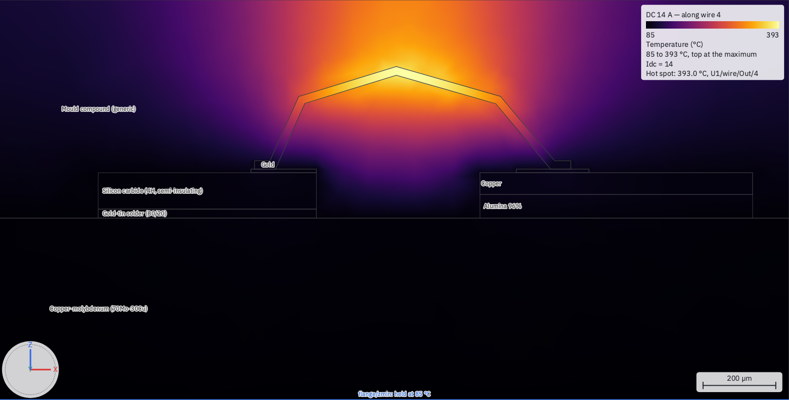
The places. These are drawn in the view but are not objects: they are never solved as metal, never snapped to, and an EM setup ignores them. Each has a group in the object tree (Heat sources, Probes, Mesh regions) whose rows select, rename, hide and delete, and a switch under 3D ▸ View. Selecting a row shows its fields in Properties, dimensions included, each a number or an expression.
- Heat source (Shift+A H, or 3D ▸ Draw ▸ Heat Source ▸ Rectangle / Polygon): drawn as a port's sheet is — put the drawing plane on the face first (Ctrl/Cmd-click it) — then named and given a default power in W. Right-click a solid, Heat Source from Solid, spreads the heat through its whole volume instead. Drawn hatched in orange.
- Probe (Shift+A T, or 3D ▸ Draw ▸ Probe ▸ Point / Spot / Line): a point on a face; a spot (its centre, then its diameter — what an IR microscope averages); or a line (two points: temperature along it). Right-click a face (Face mode) or a solid or a wire (Object mode), Add Probe, for a probe over the whole face, solid or wire. A probe may state a limit in °C; the results flag where it is crossed.
- Mesh region (Shift+A M, or 3D ▸ Draw ▸ Mesh Region): a box, drawn as a Box is, with the element size inside it — fine mesh where you put it. Drawn dashed.
Boundaries. Every face nothing names is insulated. In Face mode, right-click a face, Thermal ▸ Fixed Temperature…, Convection…, Insulated or Clear: each writes the active thermal setup (greyed, saying why, when the active setup is not a thermal one). A conditioned face is tinted — blue a fixed temperature, green convection — and listed under Thermal boundaries in the tree. Untick a boundary's row to stop drawing its tint (in this view only: the boundary still applies). Click the tint, or its row, and Properties edits it — Kind, T or h and Ambient, each a number or an expression, and Select face for the face under it. With two touching objects selected, Thermal ▸ Contact Resistance… overrides the technology's interface resistance for that contact, prefilled with the technology's value when it states one.
Contacts. Where two solids touch, heat crosses perfectly unless a resistance is stated: the technology's ThermalInterfaces give one for a pair of materials (GaN on SiC, a die attach), and a document's contact override replaces it for one contact only. The run splits the contact — each side keeps its own nodes — and joins the two through the resistance, so a clip plane through a die attach shows the temperature step. The run's notes list every contact in force, where its value came from and the area it covers.
Effective blocks (3D ▸ Draw ▸ Effective Block): a box drawn over a via field, as a mesh region is. Enabled, a thermal run replaces the board dielectric, copper planes and via barrels inside it with one block conducting (k_xy, k_xy, k_z) — hundreds of thin barrels stop forcing tiny elements. It is an approximation and is drawn disabled: enable it from its row or in Properties, which show the tensor it would carry; disabled, the geometry is solved as drawn, so comparing the two is one toggle. A box that cuts into anything else (a flange, a die) is refused, naming it. The mixture, per layer of the box (every height a replaced solid starts or stops), from the area fractions of copper, dielectric and void measured exactly over the box's footprint:
- through the layer, k_z = f_Cu·k_Cu + f_d·k_d;
- in the plane, the layer's largest phase is the matrix and the rest are inclusions (parallel cylinders) at their area-weighted k_i and fraction φ: k_xy = k_m·[(k_i + k_m) + φ(k_i − k_m)] / [(k_i + k_m) − φ(k_i − k_m)];
- the layers stack: k_z in series over their thicknesses, k_xy in parallel.
Each material's k at 25 °C is used, so the block's tensor is constant. It ignores how heat crowds into each barrel through a thin plane, which makes it run cooler than the vias drawn — measure the difference on your own board before trusting it.
Submodels. A thermal setup whose Thermal page says Submodel: cut from another thermal setup, to region a mesh region, solves only that region's box, meshed at the region's size, with its cut faces fixed to the other setup's solution; every other boundary is as written. The whole-model result is reused only when the document and every file it was solved from are as they were — a placed layout, the technology, a material library — and solved first when they are not (the notes say which, naming the file that changed). A mesh region a submodel is cut to no longer refines the whole-model run — that is what keeps it coarse. The run compares the heat crossing the cut faces with the whole model's over the same faces and warns when they differ by more than 5 % point by point: the region is too small, the fine detail changes the temperature at its edge, enlarge it. A heat source straddling the box is refused; one inside must carry the same power as in the whole model.
Symmetry. Model half (or a quarter) of a symmetric device: right-click the face you cut it on, Symmetry Plane. The
plane is drawn hatched across the model where it cuts it, labelled Symmetry X = …, and listed under Symmetry planes,
whose tick shows or hides it; select its row to move it in Properties (At, a length or an expression). It must lie on the
model's extent; it stays insulated (a condition on it is refused), and All exposed faces never
takes it. What is drawn is what is solved: give the sources the power of the modelled part. Measures read
SymmetryFactor (2 per plane) so a whole-device figure is explicit — Rth_full = (Tmax(ch) - 25) / (Pdiss * SymmetryFactor); nothing is multiplied silently. A plotted temperature is drawn mirrored across the planes (3D ▸ View ▸
Temperature ▸ Mirror Symmetric Halves turns it off), and hovering the mirrored half reads the modelled point's value and
says so.
The setup's Thermal page, top to bottom: Sources (each heat source's default, and this setup's override),
Boundaries (the list the menu writes, and All exposed faces: convection at an h and an ambient), Sweep (up to two
variables), Measures (one per line — Rth = (Tmax(die) - Tavg(flange)) / Pdiss — checked as you type), Mesh (order,
elements across a source and through the thinnest solid, grading, the solver, the convergence check), and Balance (k(T)
on or off), Submodel (above), and the three small-signal sections below — Rth matrix, Thermal impedance and
Pulse train. Under Mesh, the size of the run is estimated before anything is meshed.
Plot Temperature. A temperature picture is a field plot — a row of the tree's Field Plots group, saved with the
document, edited in the Properties Inspector (see the 3D view). After a run of the active
thermal setup, right-click a face, Plot Temperature, to add that face to the temperature plot being drawn, or start one
with it (again to take it off; several faces accumulate); 3D ▸ View ▸ Temperature ▸ All Faces draws a plot on every
exposed face, and On Clip Plane one on the clip plane's section — the way to see a channel under a field plate. The
items are greyed, with the reason, when there is no thermal result or the model has changed since it ran. The colour
range is the true minimum and maximum of what is painted — the peak is the answer, so it is never clipped — and the
legend reads °C; the plot's Fix range across the sweep (or Fix Range Across Sweep in the menu) makes it the minimum
and maximum over every sweep point, so stepping the sweep never rescales the colours. The plot's Solution is the sweep
point shown. When the run has more than one point, a sweep slider at the view's top left moves the drawn plot to
another point: one control per swept variable, labelled with its value and unit (Pdiss = 7 W). Dragging it shows the
points as it passes them, and letting go keeps the point shown as the plot's Solution, one undo step. ◀ and ▶ move one point
each. The probe table, the line plots and the hot spot follow it. Hover a painted face for the temperature there (interpolated, not the nearest
node); a ring marks the hot spot with its temperature and its object. A bond wire whose run tabulated its temperature
is coloured along its length, and hovering it names the wire and the distance along it.
Along a line. Along… on the toolbar (or 3D ▸ View ▸ Temperature ▸ Temperature Along…) takes two points and plots the temperature between them, with both end temperatures and their difference — Rth by hand, with nothing added to the document. A line probe's row in the tree plots its own, Plot T(s). Probes on the toolbar lists every probe statistic and every measure at the sweep point shown, a column per point on request, with any probe past its limit in orange.
Rth matrix, Z_th and pulses
They are read off the same mesh after the sweep, at its first point, each with every boundary made homogeneous (fixed temperatures and ambients 0) — so they are properties of the structure, not of the heatsink temperature. With k(T) on they are the small-signal response about that point's temperatures, and the notes say so.
- Rth matrix: R_ij is the rise of heat source i's place per watt in source j (every source, or the ones named). Mean
(the default) reads each source's average rise, and the matrix is symmetric — the run reports its largest asymmetry as a
check on the solve; Hottest point reads each source's maximum, which is not symmetric. The run also gives each
source's rise under the setup's own powers, R·P.
circuitrf emprints the matrix, rows and columns named. - Thermal impedance Z_th(jω), from DC over a logarithmic band (0.01 Hz to 1 MHz, 10 per decade, unless stated): every source's own place per watt in each source, and each named probe (its mean) per watt in each. Every meshed material must state DensityKgM3 and SpecificHeat; one that does not is refused, named with its objects. Right-click a heat source's or a probe's row, Plot |Z_th| or Plot Z_th phase, for the curve against log frequency.
- Foster networks. Each Z_th is fitted as Σ Rᵢ/(1 + jωτᵢ) with every Rᵢ ≥ 0 (so the network is passive) and ΣRᵢ equal
to the Rth; the fit's largest error over the band is in the notes, and above 2 % the run warns — raise per decade. Each
source's own network is written beside the result as
<result>.<source>.foster.cnl: Rᵢ ∥ Cᵢ stages between a thermal pin and a reference pin, power as current and temperature rise as voltage. Its internal nodes are not temperatures, and it is not attached to any device. The file carries a one-port bench, socircuitrf sparamon it reads the network's Z_th back. - Pulse train: a period (
1 ms,100 us), a duty, and optionally the total power during the pulse (shared by the sources in proportion to their own; empty, each at its own power). There is no transient solver. The periodic peak and the average come from Z_th solved exactly at the harmonics of 1/period, as many as it takes until each further one adds less than 10⁻⁴ of the average rise, up to the band's top. Above the last harmonic, a source's own place is carried by its Foster network. Heat from another source, or at a probe, gets nothing there: it has to travel, so it is small at high frequency. The Foster fit of such a transfer Z_th is not used: heat that has to travel arrives late, its Z_th goes negative at high frequency, and no sum of RC stages can do that. The single pulse is the train's first pulse from rest, highest before the second begins, from the same solved values. Each is added to the place's temperature with no power, for every Z_th place at every sweep point. The duty and period are expressions, so they sweep. They are rows of the Probes table, and the waveform over one period is in the result. A probe on a heat source converges slowly this way, since it has no fit of its own; the run warns when a place had not converged by the band's top.
From the command line
Every step above has a command-line spelling, and none of them needs a solver except em:
- The format.
circuitrf reference 3d-viewprints the.c3dformat, field by field, with a whole worked file. A 3D view can be written by hand, or by a script, as well as drawn. circuitrf check <path>— on the.c3d, the cell or the workspace: every object, name, expression, instance, port and setup, with each port's inferred polarity reported. The example checks clean.circuitrf explain <path.c3d>— how it elaborates: where each name's value came from, which technology each instance resolved through, every solid with its material and extent in metres, each port's contacts edge by edge, the air box, and an estimate of the problem's size.circuitrf render <path.c3d> --section xz@y=0mil -o cut.svg— a section through it;--isofor an isometric view. The pictures on this page are drawn that way. A section fills each object at its transparency;--transparency lid=80sets one (or a placed cell's, or every member of a group:--transparency stage1=40) for that picture alone, without editing the file.- Reference images are drawn by
--iso, as Copy as Vector draws them; a section draws none.checkwarns — never errs — on an image whose file is missing or will not read, a face image whose face is gone, andLockedon a sheet with no image. See Reference images. circuitrf em <path.c3d> --setup "Lid modes"— runs one setup, exactly as Run does, and writes the same files.circuitrf convert part.step -o Cell/3d/Cell.c3d— Import STEP into a new 3D view, each part's material by name or colour, or--material <part>=<material>;circuitrf convert x.c3d -o x.step— Export STEP, with the dialog's choices as flags. See convert ▸ STEP, both ways.circuitrf convert x.c3d -o x.glb— Export glTF, with--gltf-assemblyand--gltf-field <plot>; the camera is the Look's when the document saves one. See convert ▸ glTF and Exporting for another renderer.- Booleans, fillets, chamfers and Step parts by hand. The
Boolean,Fillet,ChamferandStepobjects are ordinary JSON in the.c3d, andcircuitrf reference 3d-viewprints every field; the rules for their names, faces, edges andHashare in File formats ▸ The 3D view's operations.
Keys at a glance
| Key | What it does |
|---|---|
| O, E, F, V | Select objects, edges (Edge mode, for Fillet… and Chamfer…), faces, vertices |
| B, Shift+B | The next thing behind the selection; back toward you |
| Ctrl/Cmd+A | Select every shown object (3D ▸ Select All Objects); hidden ones are left out |
| H | Hide the selection; show it if any of it is hidden (3D ▸ Hide / Show Selection). In the view or the object tree |
| Shift+A then a letter | Box, Sheet, polyGon, polyLine, cYlinder, sphEre, ellipsOid, Port, Capacitor (lumped element), Wire, Heat source, Temperature probe, Mesh region |
| W | The Wire tool; again puts it away |
| digits, Tab, Enter | Type a dimension instead of clicking |
| Esc | Back one step: the typed box, the shape, the tool, Face/Vertex/Edge mode, the selection |
| G, R, X/Y/Z | Move, rotate; hold to an axis |
| Ctrl/Cmd+D | Duplicate and move |
| Ctrl/Cmd+G, Ctrl/Cmd+Shift+G | Group the selection; ungroup the outermost selected group |
| Ctrl/Cmd+C, Ctrl/Cmd+V | Copy the selected objects; paste a 3D copy (Copy and Paste). In the view or the object tree |
| Ctrl/Cmd+E | Fit the selection; with nothing selected, everything shown |
| N, Shift+E, T | Push/pull a face; extrude a face into a new solid; Touching/Flush while aligning |
| double-click an edge | Its tangent chain (Shift adds it) |
| double-click a row in the object tree | Bring Properties forward for that row, when nothing is listed beneath it; a row that opens just opens or closes |
| M | Measure |
| Alt (Option) | Suspend geometry snapping while held |
| Ctrl/Cmd-click a face | Draw on that face's plane |
| Ctrl/Cmd while placing | The bottom-centre (die-attach) handle |
| Ctrl/Cmd+], Ctrl/Cmd+[ | Push into a placed cell, or enter a boolean to edit its operands; pop out, or leave it |
| Home or Ctrl/Cmd+0, 1–7, P, L, C | Fit; standard views; perspective; realistic view; clip plane |
| Ctrl/Cmd+=, Ctrl/Cmd+−; arrows; Shift+arrows | Zoom in, out; pan; orbit 15° |
| In the object tree: Shift-click, Ctrl-click (Cmd too on a Mac) | Select every row between; add or remove one row |
Every control, in detail
The sections above teach the editor through the example. This one is the reference: every control, in the order a pane presents them, with the rules each one follows.
- The line on the view. One line at the bottom of the view is the editor's status line: what the armed tool wants next, or the last message — a refusal and its reason, or what an edit did. Where this chapter says the status line in the 3D editor, it means that line. The clip plane cuts the model, never the drawing grid.
- Snapping. The cursor snaps to a vertex (a square marker), an edge's midpoint (a triangle), the nearest point on an edge (an ×), a face's centre (a circle) and, when nothing is within reach, the grid (a small +) — the document's snap step on the drawing plane. A marker is drawn in the colour of the material it snaps to, and in amber on the grid or on an object with no material. A vertex wins over anything else in reach, even a nearer midpoint. Snapping reaches into placed cells, so a die's pad corner is a target in its package. Only what you can see is a target: a corner hidden behind a surface is not, except inside a translucent object or with the clip plane on. The snap distance is the layout editor's, in screen pixels, so it feels the same at every zoom. The magnet on the toolbar, and 3D ▸ Snap, turn snapping on and off, and the buttons beside it turn each kind on and off; these are your settings, not the document's. Hold Alt (Option on a Mac) to suspend geometry snapping while it is held; the grid still applies. The marker's shape says what the cursor snapped to; the point itself is read with Measure (M). A ≈ before a point means it is not exactly a point of the document's database-unit grid: a corner of an object rotated by an angle that is not a multiple of 90°, or of a cell drawn at another scale.
- Drawing. Shapes are drawn on the drawing plane — XY, YZ or XZ, at an offset along
its normal — chosen with the XY / YZ / XZ buttons and the offset box on the toolbar (a bare number is the
document's unit;
25umor10milsays its own), from 3D ▸ Drawing Plane, from a face (Drawing Plane from Face on a face's menu in Face mode, or Ctrl-click a face — Cmd-click on a Mac — with a tool armed), or through a snapped point (Ctrl/Cmd+Shift-click moves the offset there and keeps the plane). Only axis-aligned faces make a plane; a tilted face is refused, naming its normal. Moving the camera never moves the plane, and a plane seen edge-on is refused rather than drawn on. The plane is remembered for the document in the workspace's window state, not in the.c3d. A faint grid lies on it, behind the objects, in steps of the document's unit — major lines every 10 minor ones, every 5 in mil and inch — spaced to stay readable at every zoom and fading away from the view's centre and when the plane is seen at a grazing angle; the lines through the origin are in the axis colours. The snap step is the Snap box beside Unit on the toolbar — the layout editor's control, with the same steps off the technology's default: pick one or type a length (2.5mil). It is saved in the document, and changing it moves nothing already drawn. The tools are on the toolbar, under 3D ▸ Draw, and at the cursor with Shift+A — then one letter: Box (corner, opposite corner, then its height), Sheet (a rectangle, two clicks), Polygon (a closed sheet, a click per vertex; click the first vertex, press Enter or double-click to close — an outline that crosses itself is refused and the crossing shown), Polyline (construction geometry; Enter or a double-click ends it, a click on its first vertex closes it) and Cylinder (centre, radius, height) and Sphere (centre, radius; centred on the plane, so the click is its centre). A box or cylinder rises along the plane's normal; near a neighbour's feature its height snaps to that feature, so a box rises to exactly the top of a pad. Every click snaps. While a shape is in progress, type a digit to enter a dimension instead of clicking — the box that opens at the cursor shows the width, depth, height or radius the next click would set; Tab moves between them, Enter accepts, Esc goes back to the mouse. An entry that is not a length stays in the box, in red, and nothing changes. Esc cancels a shape in progress; pressed again it puts the tool down. Each new object takes the material chosen on the toolbar and a name you can change (box1,sheet1, …); each is one undo step. Extrude (a sheet's menu, 3D ▸ Modify, or a polyline selected in the tree) pulls a closed polyline, a polygon or a rectangle into a prism — move to set the distance and click, or type it — and consumes the source unless K says keep it. An open polyline extrudes to a flat ribbon when it is a straight line along an axis of its plane. - Moving and copying (Object mode). The selection — objects, placed cells, or both — is
moved, rotated and copied from its right-click menu or 3D ▸ Modify. G moves it: click a base
point, then a target point, both snapped, and the selection moves by the difference — two clicks
put a pad's corner exactly on a trace's corner. Pressed with the cursor over the selection, G takes the
snapped point under the cursor as the base at once. While moving, X, Y or Z holds the move to
that axis (a snap still decides how far) and Shift+X/Y/Z to the plane across it; press the same key to
let go. Type a digit to enter the distance (
dx,dy,dz, or one distance along a held axis). R rotates about the drawing plane's normal (X, Y or Z changes the axis) through the selection's centre, or through a snapped point Ctrl/Cmd-clicked first, in 15° steps — hold Shift to turn freely, or type the angle. Rotate 90° and Mirror (across XY, YZ or XZ through the centre) act at once. Ctrl+D (Cmd+D) duplicates the selection and moves the copies; Esc cancels both. Array… makes copies along up to three axes at a pitch, shown as you type. Align lines the others up with the last one selected, by their minimum, centre or maximum on an axis. Order moves objects in the construction order — where two solids overlap, the later one wins, except that metal always wins over a dielectric whatever the order (an air object drawn after a metal still cuts a hole in it) — and the tree and the Properties panel show each object's place in it. The gizmo at the selection's centre moves it too: drag an arrow to move along that axis, or a square to move in that plane. While any of these runs nothing is changed yet; the selection moves on screen, and the document changes once, as one undo step, when you click or release. A rotation keeps an object what it was — a rotated box is still a box — and the file stores it as at most three turns. A result that is not a whole number of database units is rounded and the status line says ≈. - Editing faces and vertices (Face and Vertex modes). Right-click a face, or use 3D ▸
Modify ▸ Face. N (Move Along Normal) pushes or pulls the face: its plane moves and the faces around
it keep theirs, stretching to meet it — push a box's top up and it is still a box, only taller. It stops
just before a neighbour would shrink to nothing, and the status line names that neighbour (
'side2' would vanish at 1.2 mil); a typed distance past that point is refused rather than shortened. G moves the face freely, base point to target point, with X/Y/Z and typed distances as for objects; the faces around it tilt to follow. Shift+E (Extrude to New Solid) grows a new solid from the face along its normal — a bump from a pad, a wall from a floor — in the toolbar's material, or the source's with M; the source is unchanged. Align to Face… then a click on another face moves the object until the two are in one plane: Touching (facing each other, a die on its substrate) or Flush (the same way), T switches, and the result is shown before the click; faces that are not parallel are refused (rotate first). Copy as Sheet makes a sheet exactly on the face. Measure puts the face's area, perimeter and outward normal in Properties; Shift-click a second, parallel face for the distance between them. In Vertex mode G moves the selected vertex, Properties' Set coordinates types where it goes, and Measure From starts a measurement there. Every edit keeps the solid closed: no face is ever removed, so there is no Delete in Face mode. A face that can no longer be flat is split into flat triangles, named after it (top.0,top.1), and anything attached to the face goes to every piece. An edit that would make the solid pass through itself is drawn in red and refused, naming the faces ('top' would pass through 'bottom'); nothing changes. A shape keeps its kind for as long as it can say the result with its own dimensions — a pushed box stays a box, a prism's top moved sideways is a slanted prism — and otherwise becomes a polyhedron with the same face names; the status line says so, and Undo takes it back. A cylinder's ends move only along its axis and its side only in radius, and in Vertex mode it offers just its two cap centres, which measure but do not move: Convert to Polyhedron (Object mode; for a cylinder, choose how many flat sides) makes every vertex editable. A sphere's one face,surface, is curved, so no face edit takes it — change its Radius in Properties — and its centre measures but does not move; it is not converted to a polyhedron, and a Boolean is how to cut one. While a face or vertex is dragged only that object is redrawn, and the document changes once, as one undo step, when you click. - Dimensions as expressions. Wherever a dimension is typed — the box at the cursor while
drawing, Properties, the Array panel — you may type a name or an expression instead of a number:
w,2*w,h_sub + t_met, optionally followed by a unit (2*w mil); with none, the display unit is the expression's unit, and it is stored with the expression, so changing the display unit later moves nothing. The box shows the value as you type (= 0.254 mm), orunknown: w. Press Enter with an unknown name and a Define strip opens under the box, one row per name: a value (for a barew, the size the rubber band shows now), a unit, and whether it becomes a VAR of this 3D view or a cell parameter; Enter defines them and the shape carries on, and the definitions and the new object are one undo step. A width, depth, height, radius or extrude distance keeps its expression; a polygon's points and a move's distance are evaluated once and stored as numbers, and the box says so. A number may carry its own unit (2*w + 0.5mm); one without that is added to a name with a unit takes the box's unit, so2*w + 5withwin mil is 25 mil, and a multiplier stays a number. A lonemis milli (2mmor2metre, never2m);checkwarns about any dimension over 1 m. The Variables panel (the x button) lists each VAR with its expression, unit, value and how many fields use it, then the cell's parameters. Each row's buttons are glyphs, named by their tooltips: Set, Rename (every use is rewritten;wwis not touched by renamingw), Inline (writes the current numbers into the fields that use it, then deletes it), Promote to Cell Parameter, and Delete, last — greyed while anything uses the VAR, its tooltip naming what does. Drag the panel's left edge to widen it. A VAR with the same name as a cell parameter is linked to it: it takes the parameter's value — an instance's override, else the cell's default — and editing it edits the parameter, so the cell has one default for the name. Unlink makes it keep its own value, which then hides the parameter from this 3D view (checkwarns). Placing a cell's 3D view, an instance can override its parameters in the file ("Params"); two instances with the same values are elaborated once. Dragging a face whose size is an expression changes the name, never the field: a bare VAR is given the new value, a parameter (or linked VAR) gets a new default, and an expression linear in one name (2*w + gap) solves for that name — and every other object using it moves with it, in the preview too. A drag of anything else (2*w*l) is refused, with Replace with Number offered. A move or rotation is refused when it would change a name another object uses, because only the selection moves while you drag. - Setups (Simulate ▸ Setup Analyses… with a 3D view active, or the editor's tune button). A 3D view
carries its own EM setups, in the same form a
.cemhas, and the dialog lists them as a schematic's analyses are listed — one card each, with its kind (SP, ES, MS or EIG) and its solver and sweep: Add, Edit, Duplicate, Rename, Remove and Make Active, also on each card's right-click menu with Run. The active setup (the filled radio mark) is the one Simulate ▸ Run runs and whose air box is drawn; which one is active is remembered per user, not saved in the.c3d. Double-click a card to edit that setup in the same panel a.cemopens, less the layout row (the 3D view is the geometry) and the planar analyses (a 3D view is solved by Palace or openEMS). Every change is an edit of the 3D view: Undo takes it back and Save writes it. A static setup's terminals name their conductors by object (top, orU1/pad3inside a placed cell), because a drawn object has no net. Show 3D on a.cemwhose geometry is a.c3dopens this editor, with that.cemlisted read-only and active, so its ports and boundaries can be seen. - Ports (P in the Shift+A popup, or 3D ▸ Draw ▸ Port). A port is drawn like a sheet —
two corners on the drawing plane — or made from a face: right-click a flat, rectangular face and choose
Make Port ▸ Lumped or Wave (a wave port takes any flat face, as the rectangle round it). It takes the next free number and the last port's Z0. Which way round it
is comes from what it touches: each edge of the rectangle is tested against every conductor, and exactly
one pair of opposite edges must each touch exactly one conductor. The end that is ground — the setup's
Ground net, a placed layout's ground plane, or a PEC face of the air box — is −; otherwise the larger
conductor is. A lumped port is drawn as a checkerboard over exactly its own rectangle, − edge to + edge and
its full width, with its number and a flat arrow painted on it pointing to +; while it is being drawn the
arrow, or the reason it cannot be one, follows the cursor. Right-click a port for Flip, its kind, Z0…
and Delete. A wrong polarity turns every transmission term by 180°, so check the arrow before a run.
A wave port must lie on a face of the active setup's air box. Every setup uses every port, and a
placed cell's own ports are never used: only the parent says where a signal enters.
On a box face met by three or more conductors, or by two or more strips between the box's PEC faces, Make
Port ▸ Wave makes one port with a terminal per conductor besides the reference, named
P<n>with the next free numbers, and names the port after the face (xmin); the status line says how many terminals it made and which conductor is the reference. Such a port is one row of the tree, its tick the whole port's, with a row beneath it for each terminal: its number, name, conductor and Z0. Right-click the port for Set Reference (any conductor meeting its region; choosing a terminal's conductor swaps it with the reference), Model and Delete; with a terminal's arrow selected, the same menu adds Flip and Z0… for that terminal. Flip reverses the terminal's arrow; the reference stays the reference. - Bond wires (W, W in the Shift+A popup, or 3D ▸ Draw ▸ Wire). A wire runs between two metal
objects or sheets — a die's pad inside a placed cell to a lead in the package is the usual case, which a
.wBondcannot do because it belongs to one layout. Click any face of the object the wire starts on: each end attaches to its object's top, above the point you clicked (a side face lands just inside the top's edge; a snapped corner or face centre on a top is taken exactly). An object with no material, or an insulator, is refused with the reason. Then click the object it ends on, then move to set the loop height and click, or type it (8mil). The loop height is the assembly one: from the top of the lower pad to the top of the wire at its highest point. The status line shows it and the wire's centre-line loop height side by side, and the height you type is the height the wire measures. Before the first click the toolbar sets the diameter, the metal, how each end is bonded (a wedge lays a foot on the pad, a ball sits on it) and the section (a flat-bottomed hexagon, or round); they start from the last wire drawn. A wire's points are its whole shape: in Vertex mode its centre-line points are shown and G moves one, and its feet are put back on the pads when you let go — an end moved to where there is no pad is refused. When the pad under a wire moves, the wire does not follow, because re-routing it would change its inductance: the wire is flagged in the tree, drawn in red, and a run says which end (w3's start is no longer on a pad). Re-Seat Wire Ends (right-click the wire, or select it in the tree and use 3D ▸ Modify) moves each end up or down onto the pad now under it; a pad that moved sideways has to be reconnected by hand. Duplicate and Array… copy wires at a pitch, and a copy whose end misses a pad is still made and flagged, so a pitch error shows at once. Foot length and ball size come from the workspace's assembly rules (.wasm) unless the wire's end states a foot length, and the run says when a built-in first guess was used. - The air box (the box button). The active setup's air box, its faces tinted by boundary: PEC grey, PMC orange, symmetry hatched, and absorbing clear. It is shown until you hide it. In Face mode its faces can be picked, but only where no solid is under the cursor (B reaches one behind a solid). Right-click one for Boundary ▸ Absorbing / PEC / PMC / Symmetry and Padding…: these change the setup, not the geometry, and the status line says which setup they wrote. With no setup active they change the 3D view's own air box, and a setup added afterwards starts with it; the Properties Inspector shows the padding and faces either way.
- Boundaries on faces (Face mode). Right-click a face of a dielectric or air object for Boundary ▸ Perfect Conductor, Conductive Surface (choose the metal) or None. The face is drawn tinted and listed in the tree under its object. A boundary stays with its face through every edit, and a face that is split into pieces hands it to each. A conductor's face takes none — it is already metal — and absorbing, PMC and symmetry boundaries belong to the air box, because both solvers can state them only on the outside of the problem. Palace finds a boundary's surfaces by the face's extent and counts them, so a neighbour's face lying in the same plane and overlapping it is refused rather than guessed.
- Simulate (Simulate ▸ Run with the 3D view active, or the toolbar's Run button — the workspace toolbar's). Runs the active setup with the
same progress, Cancel and messages as a
.cem, and opens its results in the Data Display. Afterwards the run's fields are drawn by the field plots, on the geometry the run solved, and the toolbar's mesh button shows the mesh the run made, or one made with no solve; if the 3D view, or any file the run was solved from, has changed since, a selected field plot's Properties say so and name it (Fields are from the run at 14:02; 'Board.clay' has changed since) and the fields are still shown. A run keeps, beside its result, the document it solved and a hash of every file it read: each placed layout and the sub-cells it flattens, a layout's paired.wBond, each nested 3D view, the technology and the material libraries it looks through, and — for a thermal run driven from a circuit — the schematic, each sub-cell schematic and the S-parameter files it names. Editing a field plot is display and never makes a result stale. An object with no material yet — drawn as a wireframe — does not stop the run: the solver ignores it and the run's messages say so. One whose material the technology does not define does stop it.